
Quantitative UV-Vis rests on one equation linking what the instrument reads, absorbance, to what you want to know, concentration. This page explains the Beer–Lambert law formula term by term, converts transmittance to absorbance, works through concentration examples, and shows why readings leave the straight line at high absorbance.
Quick answer: The Beer–Lambert law formula is A = εbc, where A is absorbance, ε is the molar absorptivity, b is the path length and c is the concentration [1][3]. Absorbance is defined from transmittance as A = −log₁₀ T = log₁₀(I₀/I) [1][2]. A has no units; with b in centimetres and c in mol L⁻¹, ε is in L mol⁻¹ cm⁻¹ [3]. Rearranged, c = A/(εb). The straight-line relationship holds only over a limited range: one textbook keeps absorbance within 0.1–1 for a ±1–2 % relative uncertainty in concentration [4]. At high absorbance, stray light biases readings low, while the reduced signal makes noise increasingly important [1][2].
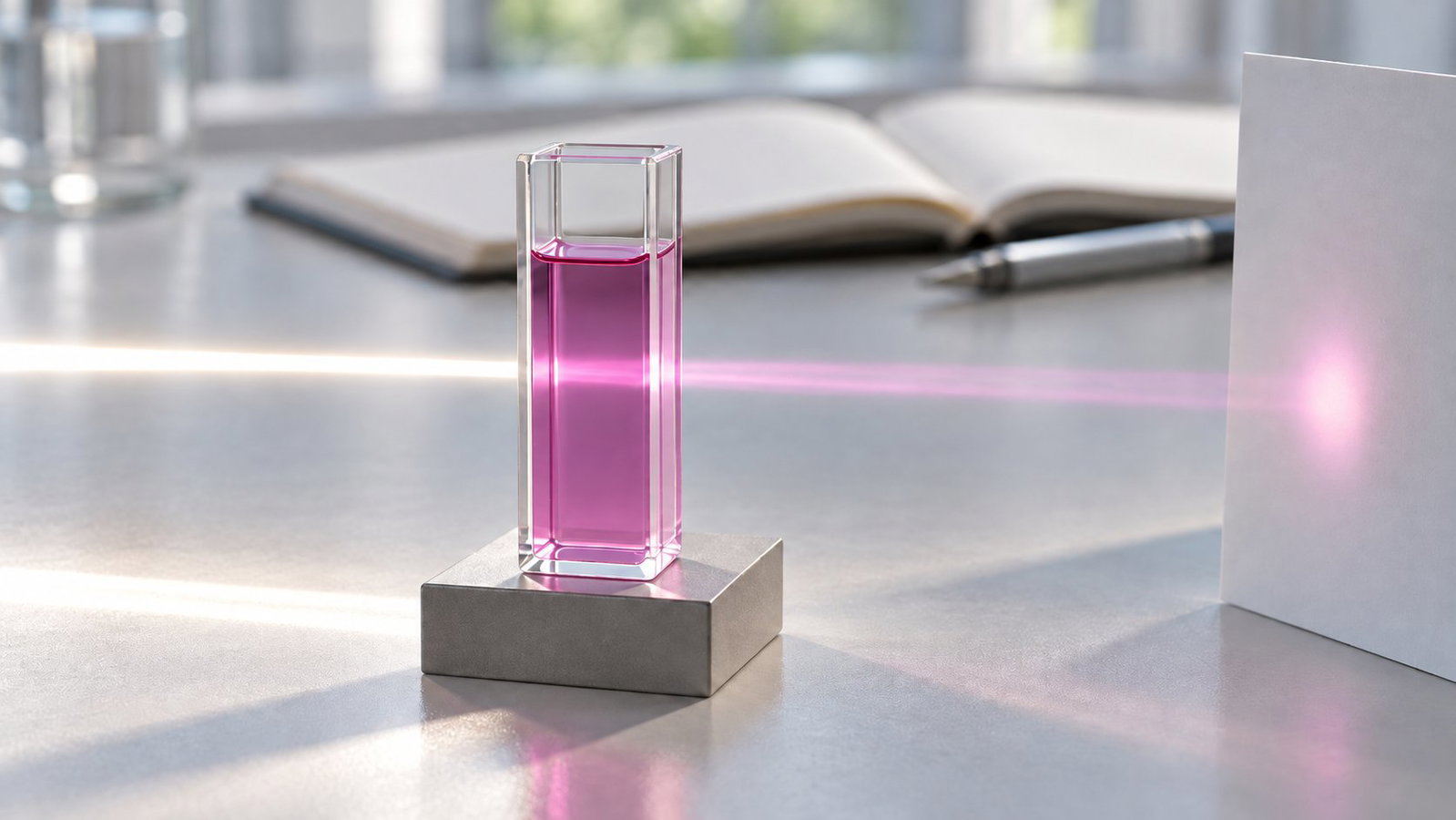
1. The Beer–Lambert Law Formula and Its Terms
The law combines two observations. The Bouguer–Lambert law describes how transmittance falls as the path length increases, T = I/I₀ = e^(−kb), where I₀ is the incident intensity, I the transmitted intensity and b the path length, usually in centimetres [1]. Beer's law says the same about concentration. Combined, they give the Beer–Bouguer–Lambert law, which becomes linear in its decadic form [1][2]:
A = −log₁₀ T = −log₁₀(I/I₀) = log₁₀(I₀/I) = εbc
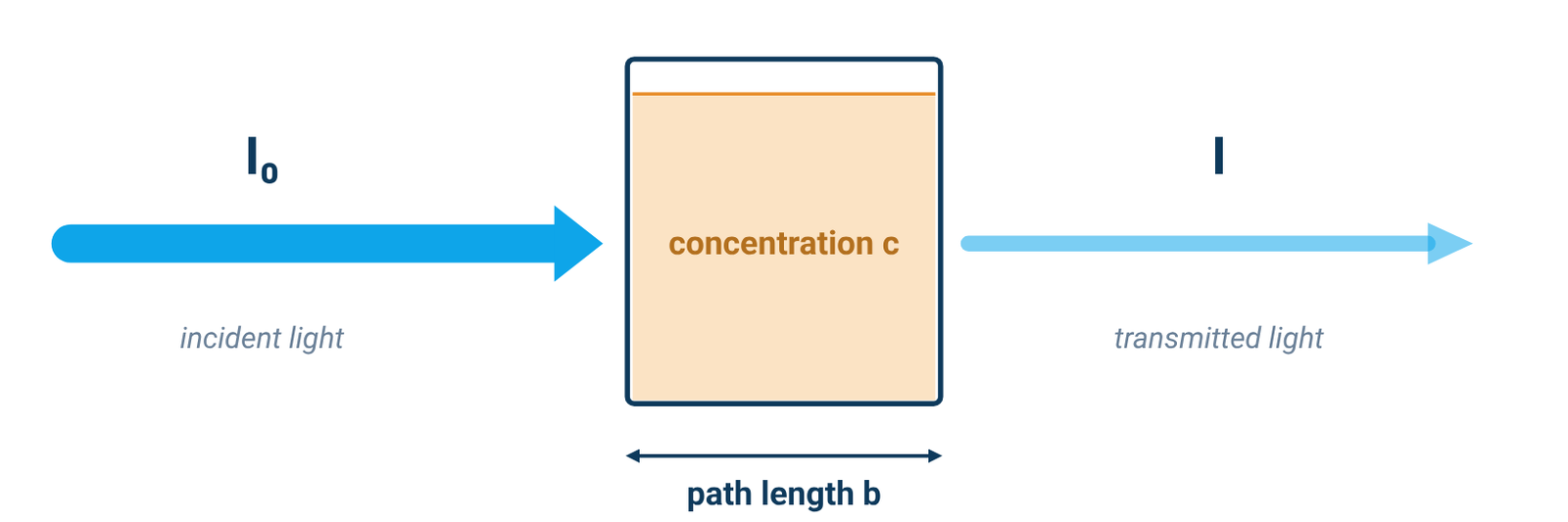
Table 1. Terms and units in the Beer–Lambert law
| Symbol | Quantity | Usual units |
|---|---|---|
| A | Absorbance | none (often written AU) |
| T | Transmittance, I/I₀ (×100 for %T) | none |
| b | Path length through the sample | cm |
| c | Concentration | mol L⁻¹ (M) |
| ε | Molar absorptivity (molar absorption or extinction coefficient) | L mol⁻¹ cm⁻¹ (M⁻¹ cm⁻¹) |
| a | Absorptivity (mass absorption coefficient), used instead of ε when c is a mass concentration (A = abc) | cm⁻¹ per concentration unit |
Sources: Owen [1], Agilent [2], Harvey [3].
ε is not a universal constant. It is characteristic of a substance under a defined set of conditions such as wavelength, solvent and temperature, and the measured value also depends partly on the instrument [1][2]. For that reason, published ε values are usually not used directly for quantitative analysis; a calibration curve is built from standards of known concentration instead (Section 8) [1][2].
2. Converting Transmittance and Absorbance
Transmittance is the fraction of light that passes through the sample, T = I/I₀, or %T = 100 × I/I₀; absorbance is A = −log₁₀ T [1][2]. Absorbance is used for quantitative work because it is normally linear in both concentration and path length, while transmittance is not [1][2].
Table 2. Transmittance and absorbance
| %T | Absorbance (A) |
|---|---|
| 100 | 0 |
| 50 | 0.3 |
| 10 | 1 |
| 1 | 2 |
| 0.1 | 3 |
| 0.01 | 4 |
Source: Agilent primer, Table 3 [2].
As Table 2 shows, each step of one absorbance unit means ten times less light reaching the detector. At A = 3, only 0.1 % of the incident light gets through [2], which is why readings at high absorbance are the hardest to make reliably (Section 6).
3. Worked Examples: Absorbance to Concentration
Worked example 1 — finding ε from a standard. A 5.00 × 10⁻⁴ M solution in a 1.00 cm cell has an absorbance of 0.338 at 490 nm. Then ε = A/(bc) = 0.338 / (1.00 cm × 5.00 × 10⁻⁴ M) = 676 M⁻¹ cm⁻¹ [3].
Worked example 2 — absorbance to concentration. A solution of the same analyte reads A = 0.228 in a 1.00 cm cell. Then c = A/(εb) = 0.228 / (676 M⁻¹ cm⁻¹ × 1 cm) = 3.37 × 10⁻⁴ M [3].
Worked example 3 — proportionality. With ε and b fixed, Beer–Lambert gives A₂/A₁ = c₂/c₁ [1][2]. Changing concentration by a factor therefore changes absorbance by the same factor, as long as the measurement remains within the method's linear range.
Worked example 4 — transmittance to absorbance. A sample that transmits 10 % of the light has A = −log₁₀(0.10) = 1; at 1 %T, A = 2 [2].
Worked example 5 — correcting for dilution. If an aliquot is diluted before measurement, determine the diluted solution's concentration from the calibration, then multiply by the known dilution factor to recover the original concentration [1].
Examples 1 and 2 are a textbook example and exercise [3]; Example 4 uses the definition of absorbance [2]. Examples 3 and 5 show the proportionality and dilution steps without adding new numerical inputs [1][2]. A real result also needs a calibration curve for your own method (Section 8).
4. Path Length and Dilution
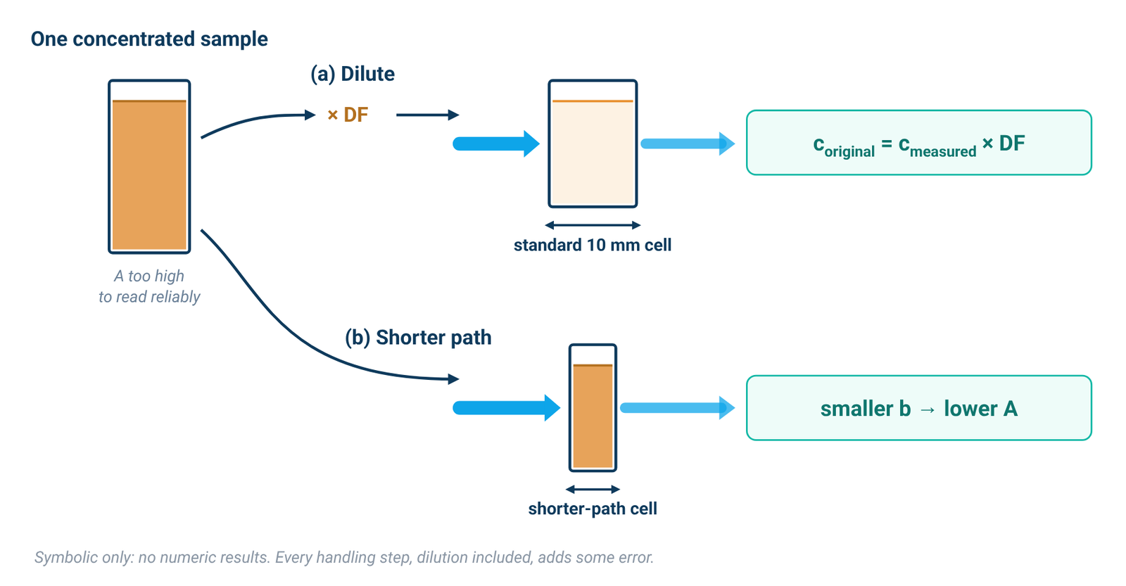
Absorbance is proportional to the path length b as well as to concentration [1][2]. Most spectrophotometers come with a holder for a standard cuvette with a 10 mm path length; longer cells need a matching long-path holder [2]. Agilent's primer suggests a short cell (5 mm or less), or dilution, for concentrated samples above about 3 absorbance units, and a long cell (up to 100 mm) for dilute samples below about 0.2 [2]. For choosing the cell material and blanking, see our cuvette guide. Quartz vs glass vs plastic cuvettes
Dilution is the easiest fix for a sample that absorbs too strongly [1]. Multiply the measured concentration by the dilution factor (Example 5). Owen notes, however, that every sample-handling step, dilution included, introduces error [1]. Measuring on the side of the band, where absorptivity is lower, is an alternative that needs excellent wavelength reproducibility [1].
On the ALab™ instruments, the standard holder is a manual four-position 1 cm holder on the single-beam SP-UV2102 and a single-position 1 cm holder on the double-beam SP-UV3101 and SP-XUV5101. These are holder descriptions, not instrument path-length specifications; path length remains a method choice as described above.
5. Linear Range vs Photometric Range
The linear range is the part of the absorbance scale where Beer's law actually holds for your instrument and method. It is not the number printed as the instrument range. Owen calls instrument range "a frequently quoted and often misunderstood specification": in most cases it is simply the numerical range an instrument can display [1]. The more useful figure is the linear dynamic range, the minimum and maximum absorbance for a given acceptable deviation from linearity [1].
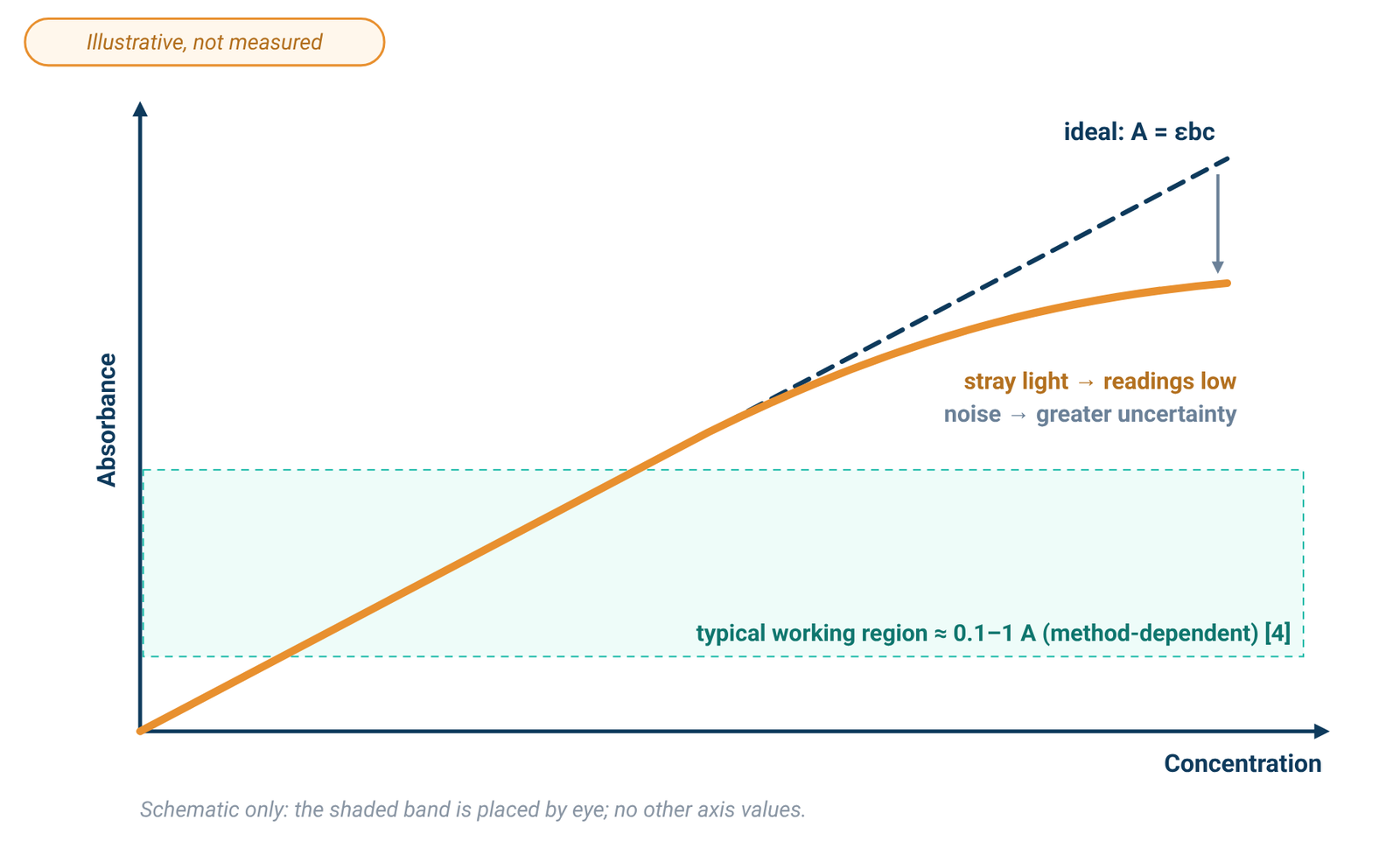
An analytical chemistry textbook states that, to obtain a relative uncertainty in concentration of ±1–2 %, the absorbance is kept within the range 0.1–1 [4]. Owen gives one worked error example: with photon noise of ±0.0004 AU and electronic noise of ±0.0001 AU, measurements from about 0.3 to 1.0 AU had the highest accuracy and precision [1]. That figure belongs to that example, not to every instrument. The linear range also depends on the method: in one textbook iron procedure, Beer's law is obeyed from 0.2 to 4.0 mg Fe/L, and samples above 2 mg Fe/L are diluted before analysis [4]. Instrument design and measurement parameters both set the maximum measurable absorbance; dilution or a shorter path brings liquid samples back into the linear range [2].
Spec sheets give a photometric range, not a linear range. The SP-UV2102 has a specified photometric range of −0.3 to 3 A and 0–9999 C (0–9999 F), and the SP-1000/1100 series is specified at −0.3 to 3.0 A and 0–200 %T. That is the specified display range, not a promise of linearity up to 3 A. Check linearity with your own standards.
6. Why High Absorbance Bends the Curve: Stray Light
Stray light is detected light of any wavelength outside the selected band [1]. It adds to the light that reaches the detector, so the measured transmittance becomes T = (I + I_s)/(I₀ + I_s), where I_s is the stray-light intensity [1]. Harvey writes the same effect as A = −log₁₀[(P_T + P_stray)/(P₀ + P_stray)] [3].
At low concentration, the stray term is small compared with the transmitted light and has little effect [3]. As concentration rises, less light passes through the sample. Stray light stays roughly constant, so it becomes the dominant term at low transmitted intensity [1]. The measured absorbance is then lower than expected, a negative deviation from Beer's law, and stray light eventually limits the highest absorbance, and so the highest concentration, that can be measured [1][3]. Agilent adds that stray light changes peak shape and makes concentration measurements unreliable [2].
Noise is a separate problem: it does not pull readings low, but it makes them less certain. At high absorbance very little light reaches the detector, so the signal-to-noise ratio falls [2], and the electronic noise term becomes significant [1], so replicate readings scatter more widely. To compare stray-light specifications between instruments, see our spec-sheet guide. Spectral bandwidth, stray light and photometric accuracy
7. Other Deviations from Beer's Law
Fundamental. Beer's law is a limiting law, valid only at low concentrations. At higher concentrations, analyte particles interact and the solution's refractive index changes, either of which can change the absorptivity [3].
Chemical. If the analyte takes part in an equilibrium, such as a weak acid and its conjugate base absorbing differently, the calibration curve can deviate in either direction unless every standard is buffered to the same pH [3].
Instrumental: bandwidth. Beer's law assumes monochromatic light. Real instruments pass a small but finite bandwidth, and polychromatic light always gives a negative deviation. The effect is smaller where ε is nearly constant across the band, which is one reason to measure at the top of a broad absorption peak [3]. Bandwidth is covered in detail in our spec-sheet guide. Spectral bandwidth, stray light and photometric accuracy
Sample: scattering. Suspended particles scatter light away from the detector, which shows up as an apparent absorbance even where nothing absorbs, and the error grows at shorter wavelengths [1]. This matters for dispersions such as graphene. Graphene concentration by UV-Vis
Mixtures. If the components do not interact, absorbances add: A_total = Σ εᵢbcᵢ [3].
8. Building a Calibration Curve and Choosing an Instrument
A Beer's law plot is a calibration curve [3]. For UV-Vis, it normally takes the form A = kc, where the slope k is the calibration factor [1]. Measure a standard or a series of standards and then the unknown on the same instrument [1], using a pure sample of the solvent as the blank [2]. Because this calibration should eliminate instrumental bias, absolute photometric accuracy matters less than photometric reproducibility. The instrument's linear range is critical, because the calibration relies on a linear relationship [1]. Make sure the unknown falls inside the concentration range your standards cover and the linearity you have checked (Section 5).
For routine quantitative work, the ALab™ single-beam, touch-screen SP-UV2102 includes quantitative measurement among its functions, with up to 1024M of internal memory for test data and working curves. Its work modes are T, A, C and E. The single-beam SP-1000/1100 series, which includes the UV models SP-UV1000 and SP-UV1100, can save up to 128 standard curves and 4,000 test results. For a double-beam option, the touch-screen SP-UV3101 uses tungsten and deuterium lamps and the SP-XUV5101 a xenon lamp. Photometric accuracy is specified at set absorbance levels; the SP-UV2102, for example, is specified at ±0.002 A from 0 to 0.5 A and ±0.003 A from 0.5 to 1 A. Those figures are tolerances at those levels, not a concentration accuracy. For beam design see single-beam vs double-beam spectrophotometers; for a full comparison see how to choose a UV-Vis spectrophotometer.
Table 3. Photometric range, photometric accuracy and standard holder
| Model | Beam | Light source | Photometric range (not a linear range) | Photometric accuracy | Standard holder |
|---|---|---|---|---|---|
| SP-UV2102 | Single Beam | tungsten and deuterium lamps | -0.3–3A, 0–9999C(0–9999F) | ±0.002A(0–0.5A) ±0.003A(0.5A–1A) | Manual 4-position 1cm holder (standard for single beam) |
| SP-UV1000 | Single Beam | tungsten and deuterium lamps | -0.3–3.0 A, 0–200%T | ±0.003 A @ 0.5 A, ±0.006 A @ 1.0 A, ±0.5%T @ 100%T | Manual 4-position 1cm holder (standard for single beam) |
| SP-UV1100 | Single Beam | tungsten and deuterium lamps | -0.3–3.0 A, 0–200%T | ±0.002 A @ 0.5 A, ±0.004 A @ 1.0 A, ±0.3%T @ 100%T | Manual 4-position 1cm holder (standard for single beam) |
| SP-UV3101 | Double Beam | tungsten and deuterium lamps | -0.3–3A, 0–9999C(0–9999F) | ±0.0015A(0–0.5A) ±0.002A(0.5A–1A) | Single hole 1cm holder (standard for double beam) |
| SP-XUV5101 | Double Beam | xenon lamp | -0.3–3A, 0–9999C(0–9999F) | ±0.0015A(0–0.5A) ±0.002A(0.5A–1A) | Single hole 1cm holder (standard for double beam) |
Source: ACS Material product specifications (October 2026). SP-UV1000 and SP-UV1100 values are for the SP-1000/1100 series. The photometric range is the specified display range; no linear range is specified for any model. Photometric accuracy is a tolerance at the given absorbance levels, not a concentration accuracy. The 1 cm figure describes the holder, not a path-length specification.
Explore the models: SP-UV2102 · SP-1000/1100 series (SP-UV1000, SP-UV1100) · SP-UV3101 · SP-XUV5101
9. Frequently Asked Questions
What is the Beer–Lambert law formula?
A = εbc: absorbance equals molar absorptivity × path length × concentration, with A = −log₁₀ T [1][3].
What are the units of molar absorptivity?
L mol⁻¹ cm⁻¹ (M⁻¹ cm⁻¹), when b is in centimetres and c in mol L⁻¹ [3].
How do I convert absorbance to concentration?
Divide by εb: c = A/(εb), as in Example 2 [3]. In practice, read the concentration from a calibration curve built with your own standards [1][2].
What absorbance range is linear?
It depends on the instrument and the method. One textbook keeps absorbance within 0.1–1 for ±1–2 % relative uncertainty [4]. The photometric range printed on a spec sheet is not a linear range [1].
Why does my calibration curve flatten at high absorbance?
Stray light can bias high-absorbance readings low [1][3], while low transmitted intensity makes noise increasingly important [1][2]. Chemical or concentration effects in the sample can also cause deviations [3]. Dilute the sample or use a shorter path [2].
Does a longer cuvette give better results?
For dilute samples, a longer path raises the absorbance and can reduce error [2]. Use the same cuvette for standards and samples [1].
10. Keep Exploring the UV-Vis Hub
- UV-Vis spectrophotometry guide: how the instrument works and what limits an absorbance reading.
- Spectral bandwidth, stray light and photometric accuracy: reading the spec sheet.
- Quartz vs glass vs plastic cuvettes: path length, cell material and blanking.
- How to choose a UV-Vis spectrophotometer: wavelength range, beam design and light source across all models.
- Single-beam vs double-beam spectrophotometers: drift, stability and when a reference beam matters.
- A260/A280 DNA and protein quantification: Beer–Lambert in practice for nucleic acids and proteins.
- Graphene concentration by UV-Vis: calibrating absorbance for dispersions that also scatter.