Graphene, graphene oxide (GO) and metal nanoparticles are routinely quantified by UV-Vis. But a dispersion is not a solution: the reading mixes absorption with scattering, and the coefficient that turns it into a concentration belongs to your sample, not to a paper. This guide explains what is measured, how published groups calibrate, and what invalidates a calibration.
Quick answer: UV-Vis graphene concentration is found from the Beer–Lambert relation A = αCl, but only with a coefficient calibrated for your own dispersion [1][2]. For a dispersion, what the instrument records is extinction, the sum of absorption and scattering [1]. Reported graphene coefficients vary with the dispersant, the nanosheet size and how the mass was measured [1], so there is no universal value. Graphene is usually read on its flat visible to near-infrared region, often at 660 nm [2][6]; the spectrum of GO changes as it is reduced [3]; and dispersions sediment over time [2][6]. Metal nanoparticles need a coefficient that matches their size, shape and surroundings [4].
1. What UV-Vis Measures in a Dispersion: Extinction, Not Absorbance
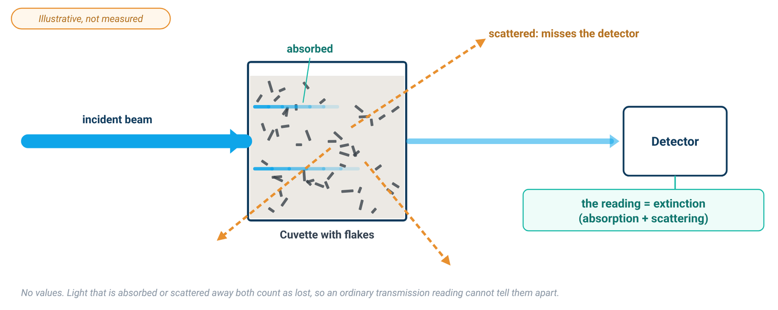
Dispersed nano-objects scatter light strongly. Backes and co-workers put it plainly: almost all experiments on liquid-exfoliated graphene actually measure the extinction of the dispersion, and extinction is what most researchers mean when they quote the "absorbance" of nanoparticulate dispersions [1]. Extinction is the sum of absorbance and scattering (Ext = Abs + Sca), so the extinction coefficient is the sum of an absorption coefficient and a scattering coefficient, ε(λ) = α(λ) + σ(λ) [1]. Both α and σ, and therefore ε, can depend on nanosheet size as well as on wavelength [1].
From the instrument side, scattering produces an apparent background absorbance, because light is deflected at an angle instead of passing through to the detector [5]. Small particles scatter roughly as 1/λ⁴ (Rayleigh) and large ones as 1/λ² (Tyndall), so the scattering error grows toward shorter wavelengths [5]. Filtering removes scattering but is not always practicable [5], and in a nanomaterial dispersion the scatterers are the analyte itself.
The true absorbance of a dispersion can be measured by acquiring the spectrum with the cuvette inside an integrating sphere, where all scattered light is collected; together with the ordinary extinction spectrum, this gives the scattering spectrum [1]. This is a research set-up (Backes used a home-built holder at the centre of the sphere) [1]. For routine work the consequence is simpler: in an ordinary transmission measurement, the coefficient you use is an extinction coefficient, and it must have been measured the same way as your samples.
2. Graphene: Why 660 nm, and Why the Coefficient Is Yours
The spectrum of liquid-exfoliated graphene is featureless in the visible to infrared region, as theory predicts [6]. In surfactant–water dispersions, Lotya and co-workers found the spectrum flat and featureless everywhere except below 280 nm, where a strong band scaled with the surfactant concentration rather than with the graphite concentration [2]. Early liquid-exfoliation work read the flat region at 660 nm [2][6]. Backes and co-workers later showed that the coefficient on the high-wavelength plateau is relatively independent of nanosheet size and thickness, and used 750 nm [1]. Reading on the plateau keeps clear of the surfactant band and of the region where scattering is strongest [2][5].
Published coefficients do not agree. Table 1 lists values printed in two of the cited papers, only to illustrate the spread.
Table 1. Reported graphene coefficients (examples from the literature)
| Source | Dispersion | Wavelength | Coefficient | How the mass concentration was found |
|---|---|---|---|---|
| Lotya et al. 2009 [2] | graphite exfoliated in SDBS/water, after centrifugation | 660 nm | α = 1390 mL mg⁻¹ m⁻¹ ("absorption coefficient") | filtration onto an alumina membrane and weighing on a microbalance; TGA showed 64 ± 5 % of the film was graphitic, the rest residual surfactant |
| Backes et al. 2016 [1] | liquid-exfoliated graphene in aqueous sodium cholate, several size fractions | 750 nm | ε750 = 5450 L g⁻¹ m⁻¹ (extinction coefficient) | filtration and weighing after washing; residual surfactant measured by TGA |
| Backes et al. 2016 [1] | as above, measured inside an integrating sphere | 750 nm | α750 = 4861 L g⁻¹ m⁻¹ (absorption coefficient, mean) | as above |
Examples from the literature; not transferable to your sample. Values and units from each source; 1 mL mg⁻¹ m⁻¹ is numerically equal to 1 L g⁻¹ m⁻¹. The rows differ in dispersant, wavelength and measurement geometry, so they are not directly comparable.
Backes and co-workers explain the spread [1]: different values have been reported for different stabilising dispersants; the spectra depend on nanosheet size and thickness, especially at low wavelength, so a coefficient is not necessarily size-independent at every wavelength; and residual solvent or surfactant on the graphene may not have been accounted for in the mass measurement. They also note that the coefficient used to quantify graphene is an extinction coefficient, although it is usually called an absorption coefficient [1].
A coefficient from another paper, dispersant or wavelength is not your coefficient. A commercial dispersion supplied at a nominal concentration, such as a graphene dispersion in water, is no exception: the nominal value describes the product as supplied and is not a UV-Vis calibration standard for the diluted or processed sample you measure.
3. Graphene Oxide: The Band Moves as GO Is Reduced
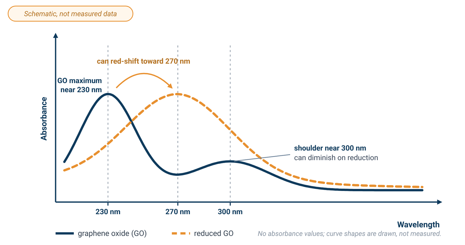
Rommozzi and co-workers describe the spectrum of an aqueous GO dispersion as a maximum at around 230 nm, attributed to π→π* transitions of aromatic C=C bonds, with a shoulder at around 300 nm attributed to n→π* transitions of C=O bonds [3]. During chemical reduction in their glucose–ammonia system, used to prepare rGO for an rGO/TiO₂ photocatalyst, the 300 nm shoulder gradually disappeared as oxygen was removed, while the 230 nm maximum gradually red-shifted to around 270 nm [3]. They also report a rise in absorbance over time in that system; treat this as one study’s observation, not a general rule for GO.
Because the band position, and possibly the absorbance, can change with reduction, a calibration made on as-made GO cannot be assumed to hold after reduction. The change is gradual [3], so calibrate on the material in the state you will measure it. The same applies to a commercial graphene oxide dispersion: dilute it in the medium you will use and build your own calibration.
GO's main band sits in the UV. Glass absorbs strongly below 320 nm and is not suitable there, while fused quartz cells are reasonably transparent down to about 210 nm [5]. Use quartz for GO work and blank with the same medium; our quartz vs glass cuvette guide covers cell cut-offs and blanking.
4. Building a Sample-Specific Calibration
The coefficient comes from the Beer–Lambert relation, A = αCl, where C is the concentration and l the path length [2]; our Beer–Lambert law guide covers units and the linear range. The groups cited here built their calibrations in much the same way [1][2][6]:
- Prepare a stock dispersion with the same solvent or surfactant solution, and the same processing, as the samples you will measure [2][6].
- Find its mass concentration independently. Filter a measured volume onto a membrane of known mass, wash and dry the film, and weigh it [1][2]. Correct the mass for residual surfactant, measured by TGA [1][2], or for residual solvent [6].
- Dilute the stock serially with the same surfactant solution or solvent [2].
- Read each dilution at the chosen wavelength against a blank of that same medium.
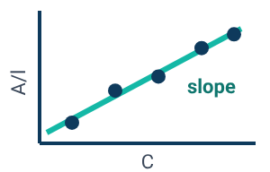
- Plot absorbance per unit path length (A/l) against concentration. The slope of the straight-line fit is the coefficient for that dispersion [2][6].
- Use it only for samples prepared the same way.
In Lotya's calibration the line did not pass through zero; the intercept was attributable to residual surfactant [2], a reminder that the medium contributes to the reading. Keep the readings in the working range of your instrument, and dilute a sample that reads high rather than extrapolating beyond the highest calibration point (see the linear range).
Recalibrate when the dispersant or the nanosheet size distribution changes [1], or when GO has been reduced [3].
5. Sedimentation and Time
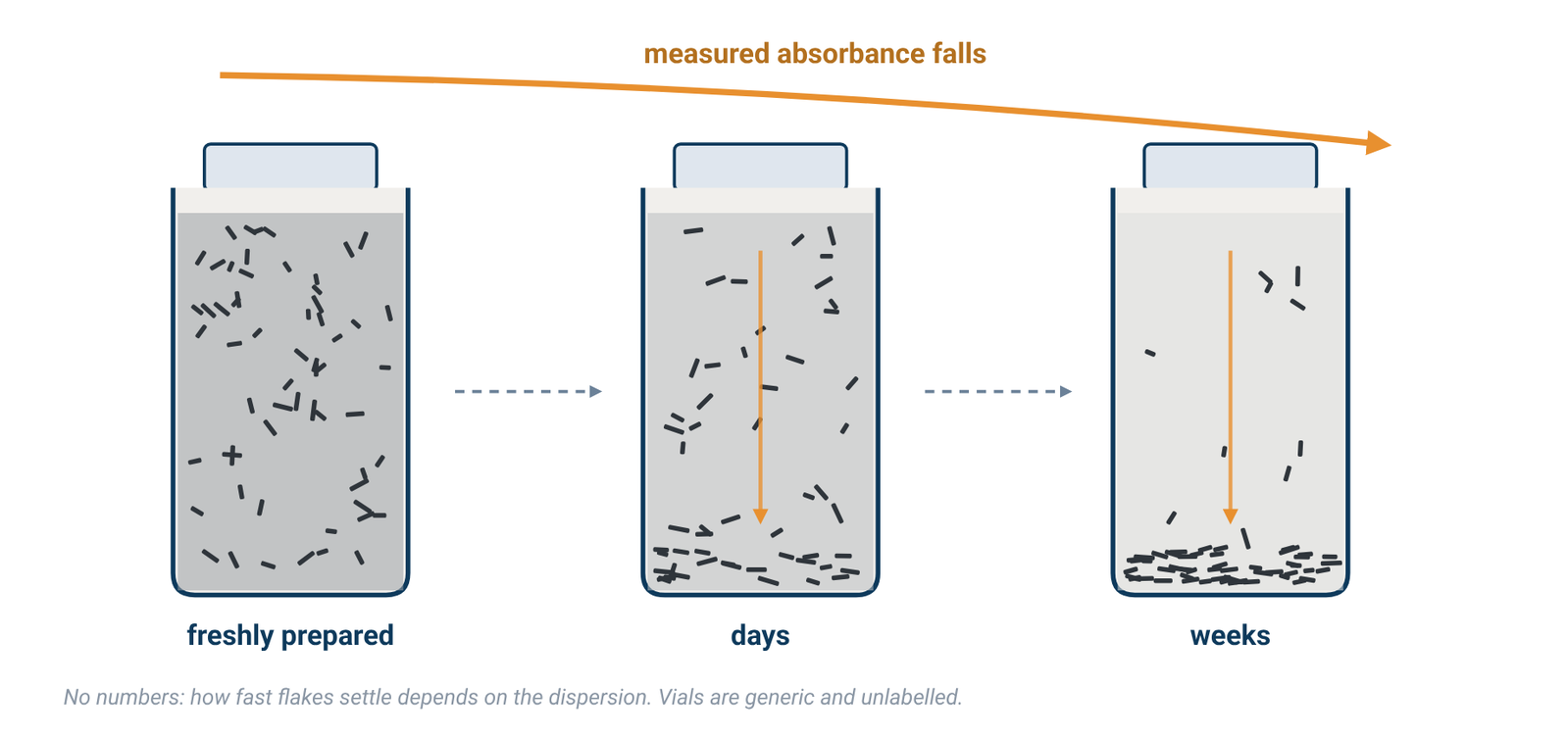
Lotya and co-workers monitored the absorbance of an SDBS-stabilised graphene dispersion at 650 nm over time: it fell steadily, indicating that about two thirds of the material sedimented; a fit showed 35 wt% of the sample stable over 35 days, while medium and large flakes sedimented out over about six weeks [2]. Hernandez and co-workers reported moderate sedimentation and aggregation within three weeks of centrifugation, although their dispersions remained of high quality for at least five months [6]. These timescales belong to those dispersions; yours may differ.
Note the time since the dispersion was prepared or centrifuged, measure standards and samples on a similar schedule, and repeat readings if stability matters.
A double-beam instrument does not remove this effect. The dual-beam design was developed to compensate for changes in lamp intensity between the blank and sample measurements [5]; it does not compensate for a sample-side concentration change caused by material settling in the cuvette. Beam design is covered in single-beam vs double-beam spectrophotometers.
6. Metal Nanoparticles: The Coefficient Depends on Size, Shape and Surroundings
Haiss and co-workers note that the influence of particle size, shape, dielectric environment and surface coatings on the extinction and scattering cross sections of small metal particles has been discussed in the literature [4]. Their method for spherical gold nanoparticles in water works in two steps: first estimate the particle diameter, for example from the position of the surface plasmon resonance or from the ratio of the absorbance at the resonance peak to that at 450 nm; then calculate the concentration from the absorbance at 450 nm using the extinction efficiency for that diameter [4].
The authors are explicit about the limits. The influence of a coating and of the surrounding medium on the extinction efficiency, and hence on the absorbance, cannot be neglected, and their equations or fit parameters have to be modified for other dielectric environments [4]. The calculations assume monodisperse, perfectly spherical particles, while real samples have distributions of size and shape that can broaden or shift the plasmon band [4]. For other materials and environments, they encourage readers to develop their own calibration curves [4]; for coated, non-spherical or non-aqueous particles, use a coefficient derived for that system or calibrate.
7. Measuring Well
Blank with the dispersion medium. In surfactant dispersions the surfactant itself absorbs strongly below 280 nm [2], so the blank should be the same solvent or surfactant solution at the same concentration. Cells and blanking are covered in our cuvette guide.
Stay in the working range. Stray light affects the linear relationship between absorbance and concentration most strongly at high absorbance [5], so dilute concentrated dispersions rather than reading them neat. The photometric range printed on a specification sheet is not the linear range, and no specification gives a concentration accuracy; see spectral bandwidth and stray light.
Bandwidth is not the limit. Absorption bands of samples in solution are normally broad, and a spectral bandwidth of 2 nm is more than adequate for bands 20 nm wide or more [5]. The graphene spectrum is featureless across the visible region [6], so a narrower bandwidth is not needed for these readings.
For wavelength range, beam design and light source, see how to choose a UV-Vis spectrophotometer.
8. Instruments for Dispersion Work
Any UV-Vis spectrophotometer covering your wavelengths can follow this method; the calibration, not the instrument, turns a reading into a concentration. The ALab™ double-beam SP-UV3101 has a specified wavelength range of 190–1100 nm, which covers the GO band near 230 nm and the 660–750 nm plateau used for graphene in the literature; it uses tungsten and deuterium lamps and comes with a single-position 1 cm holder as standard. The double-beam SP-XUV5101 has the same 190–1100 nm range and uses a xenon lamp. The single-beam SP-UV2102 also covers 190–1100 nm, uses tungsten and deuterium lamps, and comes with a manual four-position 1 cm holder as standard.
The listed spectral bandwidths are 1.0nm for the SP-UV3101 and SP-XUV5101 and 2.0nm for the SP-UV2102; for the broad spectra of these dispersions either is adequate [5]. The listed stray-light values are ≤0.02%T @ 220,360nm for the SP-UV3101 and SP-XUV5101 and ≤0.05%T @ 220,360nm for the SP-UV2102 (Table 2). ACS Material makes no graphene, nanoparticle, scattering-correction or concentration claim for these models; the calibration is yours.
Table 2. Specifications of the models mentioned
| Model | Beam | Light source | Wavelength range | Spectral bandwidth | Stray light | Standard holder |
|---|---|---|---|---|---|---|
| SP-UV3101 | Double Beam | tungsten and deuterium lamps | 190–1100 nm | 1.0nm | ≤0.02%T @ 220,360nm | Single hole 1cm holder (standard for double beam) |
| SP-XUV5101 | Double Beam | xenon lamp | 190–1100 nm | 1.0nm | ≤0.02%T @ 220,360nm | Single hole 1cm holder (standard for double beam) |
| SP-UV2102 | Single Beam | tungsten and deuterium lamps | 190–1100 nm | 2.0nm | ≤0.05%T @ 220,360nm | Manual 4-position 1cm holder (standard for single beam) |
Source: ACS Material product specifications (October 2026). No graphene, nanoparticle, scattering-correction or concentration claim is made for these models. Either bandwidth is adequate for broad dispersion spectra [5]. The 1 cm figure describes the holder, not a path-length specification.
9. Frequently Asked Questions
What wavelength is used for graphene concentration?
Early liquid-exfoliation studies used 660 nm, on the flat part of the spectrum [2][6]; Backes and co-workers used 750 nm, where the coefficient is relatively independent of nanosheet size [1]. Whichever you choose, calibrate at that wavelength.
Is there a standard extinction coefficient for graphene?
No. Reported values vary with the dispersant, nanosheet size and how residual surfactant or solvent was handled in the mass measurement [1]. Use published values only as a guide, and calibrate your own dispersion.
Why is my graphene "absorbance" higher at short wavelengths?
Part of the reading is scattering, which grows toward shorter wavelengths [5]; in surfactant dispersions the surfactant also absorbs strongly below 280 nm [2]. The instrument records extinction, absorption plus scattering [1].
How do I measure graphene oxide concentration by UV-Vis?
Build a calibration on your own GO: find the mass concentration of a stock independently, dilute it in the same medium, and read against a blank of that medium in quartz cells [5]. GO's main band is near 230 nm with a shoulder near 300 nm [3].
Does reducing GO change the calibration?
Do not assume that an as-made GO calibration still applies after reduction. In the cited reduction study, the 300 nm shoulder disappeared and the maximum shifted toward 270 nm [3], so calibrate the material in the state you will measure it.
Can I measure gold nanoparticle concentration by UV-Vis?
Yes, for spherical gold particles in water, using a size-dependent extinction efficiency once the size is known [4]. Coatings, other media and non-spherical shapes change the relationship [4].
10. Keep Exploring the UV-Vis Hub
- UV-Vis spectrophotometry guide: how the instrument works and what limits an absorbance reading.
- Beer–Lambert law formula: A = εbc, units and the linear range.
- Quartz vs glass vs plastic cuvettes: cell material, path length and blanking.
- Spectral bandwidth, stray light and photometric accuracy: reading the spec sheet.
- Single-beam vs double-beam spectrophotometers: what a reference beam does and does not correct.
- How to choose a UV-Vis spectrophotometer: wavelength range, beam design and light source across all models.