
A graphene fiber lies on the bench. It is nineteen hundred micrometers long and twenty-eight micrometers across — thinner than a human hair, invisible against a white page. Somebody needs to know how well it conducts heat, and they need a number with an uncertainty attached to it. Most conventional bulk and planar thermal measurement methods are unsuitable for a specimen of this geometry: there is no flat face to press a sensor against, no volume to flash with a laser, not enough material to instrument. This guide is about the family of methods that do work at this scale, why they work, what they cost you in sample preparation, and how to read the number that comes out the other end.
1. Three numbers that describe heat flow
Ask three engineers for “the thermal property” of a material and you will get three different quantities back. That is not sloppiness; it reflects the fact that heat flow in a solid is governed by two independent physical capacities — the ability to transport energy and the ability to store it — and different applications care about different combinations of the two.
Thermal conductivity k answers a steady-state question: once temperatures have settled, how much power crosses a unit area per unit temperature gradient? It is the number you want when sizing a heat spreader that runs continuously. Volumetric heat capacity ρcp answers a storage question: how much energy does a cubic meter absorb per degree of temperature rise? It is what buffers a transient load. Thermal diffusivity α answers a timing question: how quickly does a thermal disturbance propagate? It governs how fast a device reaches equilibrium after a power step, and it is the natural output of diffusion-based transient measurements such as TET, because time is what those measurements actually observe.
The relationship α = k / ρcp means any one of the three can be computed from the other two. In practice this asymmetry matters enormously. A diffusion-based transient method such as TET determines α directly from the time response; reporting a conductivity from it requires an independently known density and specific heat. For a well-characterized bulk material that is trivial. For a porous carbon fiber, a wet-spun graphene filament, or a nanocomposite of uncertain packing density, ρcp can carry more uncertainty than the diffusivity measurement itself. Whenever you see a conductivity quoted for an exotic low-dimensional material, it is worth asking where the ρcp came from.
There is a fourth quantity that does not belong to the material at all, and it ruins more measurements than any other single effect: interfacial thermal resistance (ITR, sometimes thermal boundary resistance). Wherever two materials meet, phonons and electrons crossing the boundary are partly reflected, producing a temperature discontinuity for a given heat flux. How much it matters depends on contact area, surface condition, pressure and the intrinsic resistance of the adjoining layers — it can dominate a nanoscale heterostructure and an assembled macroscale thermal-interface stack alike: recent work on monolayer WSe2 on SiO2 resolved this boundary resistance by Raman probing while explicitly accounting for optical–acoustic phonon non-equilibrium1, and measurements on single-walled carbon nanotube bundles against SiO2 below 8 nm found the interfacial resistance following a T−n temperature dependence with n in the range 2.4–2.562. The same caution applies to heat capacity: absolute and differential calorimetric determinations of a single graphite specimen can be compared against one another precisely because the material is well characterized3, and no such anchor exists for most novel low-dimensional materials. Any technique that puts a sensor in contact with the sample is measuring the sample and its interfaces; techniques that heat the sample from within, as the electro-thermal family does, sidestep a large part of that problem.
2. Eight methods, one decision
There is no universal thermal measurement. What exists is a set of techniques, each of which trades sample preparation effort against applicability and uncertainty. The decision is driven less by the material than by its geometry: is it a bulk block, a supported film, a suspended membrane, or a free-standing wire? The table below summarizes the landscape, following the classification given in a recent review of transient electro-thermal metrology4.
| Method | Suits | Sample structure | Prep effort | Principal limitation |
|---|---|---|---|---|
| TET | Wires, fibers, thin films, mm down to nm | Suspended | Low | Short samples of very high conductivity become difficult |
| 3ω | Thin films | Supported or suspended | Moderate–high | Needs a patterned or transferable heater/thermometer line; interpretation depends on substrate and multilayer modeling |
| TDTR | 2D materials, films | Supported | Low–moderate | Complex optics; standard implementations use a metal transducer layer and a very smooth surface |
| Suspended micro-bridge | 2D materials, nanofilms, nanotubes | Suspended | High | Contact resistance hard to evaluate accurately; low throughput |
| Raman thermometry | 2D materials, films, nanowires, bulk | Suspended or supported | Low–moderate | Needs a measurable, temperature-sensitive Raman mode; absorbed power, spot size and phonon non-equilibrium can dominate uncertainty |
| Transient plane source (hot disk) | Bulk, thick films, powders, pastes, liquids | Supported | Low–moderate | Sensor–sample contact resistance; needs at least one flat surface |
| Electron-beam self-heating | 2D materials, nanowires, films | Suspended | Moderate | Weak signal on thin samples; demands flat, clean surfaces |
| T-bridge | 2D materials, nanowires, films | Suspended | Moderate–high | Contact resistance components difficult to separate |
Classification after the comparative summary in reference 4. “Prep effort” refers to the work needed to get a specimen into measurable form, not to instrument cost or operator skill.
Each of these methods has its own founding literature, and it is worth going to the source rather than to a summary. The flash method was introduced in 1961 and remains the most widely used route to the diffusivity of a bulk solid: a short, intense light pulse is absorbed at the front face of a disc, and the rear-face temperature history gives diffusivity from the shape of the transient, while calibrated energy input or comparison against a reference specimen can support a heat-capacity determination; conductivity then follows once density and heat capacity are known5. The 3ω method was developed for dielectric solids between 30 and 750 K, using an AC-driven metal line as both heater and thermometer and rejecting black-body radiation error to below 2 % even at 1000 K6; it was later extended to specific heat as well as conductivity7, and adapted into a four-point variant capable of measuring an individual carbon nanotube8. The suspended micro-bridge approach uses a microfabricated device with separate heating and sensing membranes to obtain thermal and thermoelectric properties of a single one-dimensional nanostructure9. Broader surveys of the low-dimensional measurement landscape10 and of resistance-thermometry approaches in particular11 are useful if you want the field mapped by authors with no stake in any one technique.
Two entries deserve comment because they are the ones most often proposed as alternatives for low-dimensional samples. The 3ω method is the workhorse for supported thin films and can extract both in-plane and cross-plane properties, but it requires a heater/thermometer line that is either patterned lithographically or provided by the film itself, and interpretation leans on modeling the substrate and any intervening layers — which is why it becomes awkward for few-layer 2D materials. Raman thermometry is attractive because it is contactless and needs almost no fabrication, but it depends on two quantities that are individually hard to pin down: the Raman temperature coefficient of the material and the fraction of incident laser power actually absorbed. Worse, treating the Raman shift as a single sample temperature implicitly assumes optical and acoustic phonons are in equilibrium. They are not always: distinct optical and acoustic phonon temperatures have been resolved experimentally in nanometer-thick suspended WS212, and neglecting the difference leads to substantial overestimation of the temperature rise, and therefore to an underestimate of conductivity. Energy-transport-state resolved Raman (ET-Raman) was developed specifically to break this degeneracy by comparing steady-state and transient heating states rather than relying on an absolute temperature calibration13; a critical review of the whole Raman-based family sets out where each variant remains vulnerable14.
None of this makes Raman or 3ω bad methods. It makes them methods with a domain. If your sample is a supported dielectric film on a smooth substrate, TDTR is likely the right answer. If it is a bulk polymer block, transient plane source will give you a result in minutes. The techniques described in the rest of this guide occupy a specific and, until recently, poorly served corner of that space: free-standing one-dimensional and quasi-one-dimensional samples, where the specimen can be suspended between two electrodes and used as its own heater and its own thermometer.
3. The transient electro-thermal technique
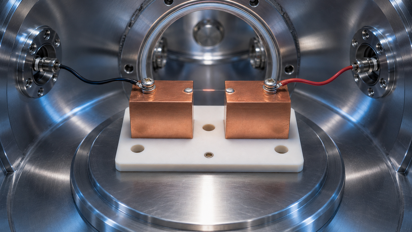
The transient electro-thermal (TET) technique was developed in 2007 to characterize exactly the class of sample described above15. Its arrangement is disarmingly simple. The specimen is suspended across a trench between two electrodes — aluminum or copper, chosen for high thermal conductivity so that they can be approximated as isothermal boundaries within the measurement model — and bonded with silver paste to secure both electrical and thermal contact. The chamber is evacuated to suppress convection. A step DC current is then passed through the sample. Joule heating raises its temperature; the temperature rise changes its electrical resistance; the resistance change appears as a time-varying voltage across the specimen. That voltage trace is the entire measurement.
What makes this work is the aspect ratio. Because the specimen is far longer than it is thick, heat conduction is effectively one-dimensional along its length, and the electrodes hold both ends at ambient temperature. Solving the one-dimensional heat equation with those boundary conditions using the Green’s function method yields a normalized temperature rise T* that depends on time only through the grouping αt/L2 — the Fourier number4,15:
T* = (96/π4) Σm=1∞ {1 − exp[−(2m−1)2π2αt/L2]} / (2m−1)4
That universality is conditional, and the conditions deserve stating plainly: one-dimensional axial conduction, properties approximately constant across the temperature excursion, a small rise with a near-linear resistance–temperature relation, both ends approximately isothermal, and convection, radiation, coating and contact effects either negligible or corrected. Inside those conditions the result is powerful: the shape of the normalized curve is universal. It does not depend on how much power you injected, on the sample’s resistance, or on its cross-section — only on α and the suspended length L. In a calibrated imaging setup L can be measured to sub-percent relative uncertainty, so the diffusivity follows from the timing of the curve alone. There is no need to know the absorbed power in absolute terms, which is precisely the quantity that limits the accuracy of optical techniques.
A family, not a single technique
What is described above is one member of a family. The architecture separates cleanly into two independent choices — how you deposit energy into the sample, and how you read its temperature — and several combinations of optical or electrical excitation with resistance-based or optical readout have been demonstrated and validated. Substituting a laser for the step current gives the transient photo-electro-thermal (TPET) technique, which retains resistance thermometry but heats optically16; because the beam can be shaped into a narrow line and scanned, it also answers a question TET cannot answer about itself, namely whether local variations in electrical resistance along the specimen bias the result. Scanning a 0.1 mm line focus along a graphene fiber showed the extracted diffusivity essentially constant except very near the ends17,18, where the reduced thermal resistance to the electrodes demands higher laser power and can perturb the boundary condition the model assumes. What that establishes is narrower than it first looks: the linearized reduction is robust against where along the mid-span the excitation lands. It does not make optical and Joule heating equivalent — in the same work the two routes differed by roughly 7.1 %, attributed to the higher overall temperature rise under laser heating (about 7 K against 2.2 K) combined with the temperature dependence of diffusivity, and to a slightly different choice of steady-state voltage18. Two independent excitation routes agreeing to within a few percent is a useful cross-check, not evidence that either is exact.
Other members swap the readout instead. Optical heating and electrical thermal sensing (OHETS) applies modulated optical heating with electrical detection19. Pulsed laser-assisted thermal relaxation (PLTR) drops the steady-state requirement altogether and reads the relaxation after a pulse, which suits samples that cannot tolerate sustained heating20. A steady-state electro-Raman-thermal variant replaces the resistance thermometer with the Raman shift21, and a Johnson-noise implementation uses the sample’s own thermal noise as the temperature probe, removing the need to inject a sensing current at all22.
The family also had to be extended in a less visible direction: not all materials have a resistance that varies linearly with temperature. In semiconductors the temperature coefficient of resistivity can vary strongly, and can even change sign, because carrier concentration and scattering time respond to temperature in opposite directions. When that happens the voltage trace stops being monotonic and no single-exponential model will fit it. Extending the physics to a higher-order dependence of resistivity on temperature yields a multi-exponential form that recovers a smooth, continuous diffusivity through the transition — behavior first characterized on anatase TiO2 nanowires23 and later applied to graphene films crossing a semiconductive-to-metallic transition4.
From a voltage trace to a diffusivity
Three approaches have historically been used to extract α from the transient. Early-stage linear fitting uses only the first instants of the rise, where the temperature climbs almost linearly; it is fast but systematically underestimates α because very few points fall inside the genuinely linear window. The characteristic point method exploits the fact that sensitivity to α is maximized at a single point on the curve, T* = 0.8665, corresponding to a Fourier number of 0.2026; the diffusivity then follows directly as α = 0.2026L2/tc15. It is accurate but hostage to how precisely that one point can be located in noisy data. Global least-squares fitting uses the entire trace and achieves the best agreement, but it requires identifying the heating onset and the steady-state voltage and normalizing the data — each step an opportunity to introduce error.
A fourth route removes most of those opportunities. Rewriting the series in terms of the remaining distance to steady state, and using Σ(2m−1)−4 = π4/96, gives
1 − T* = (96/π4) Σm=1∞ exp[−(2m−1)2π2αt/L2] / (2m−1)4
The higher modes decay as exp(−9π2Fo), exp(−25π2Fo) and faster, so at late times only the first eigenmode survives:
1 − T* ≈ (96/π4) exp(−π2αt/L2), 96/π4 ≈ 0.9855
That leading amplitude is not unity, and writing it as though it were is a small but real sloppiness. It does not touch the result, because taking the logarithm turns every multiplicative constant — the modal amplitude, and the electrical scaling between normalized temperature and measured voltage — into an additive term that lands in the intercept:
ln |V − V1| = −π2αt/L2 + D
The slope carries the diffusivity; the intercept D absorbs the modal-amplitude factor and the voltage scaling, and is discarded. Dividing the slope by the known π2/L2 gives the thermal diffusivity. The strength of that linearity, and its robustness against where along the specimen the heating is applied, has been examined systematically in the peer-reviewed literature17. This linearization, and the automated determination of thermal characteristics that it enables, is the subject of U.S. Patent No. 12,372,489 B2, granted to ACS Thermal LLC on 29 July 202518. The advantage is not merely aesthetic. A linear regression yields a slope and its standard error from the same fit — a statistic that describes the regression only, not the measurement as a whole — whereas uncertainty in a non-linear regression must be estimated from the covariance matrix under a local-linearization assumption that weakens when the model is strongly non-linear. It is also markedly less sensitive to where the fit begins: applying the transformation to graphene-fiber data with no data excluded, with points below T* = 0.05 excluded, and with points below T* = 0.1 excluded returns 9.62×10⁻⁷, 9.62×10⁻⁷ and 9.61×10⁻⁷ m2·s−1 respectively18 — a spread of 0.1 %, against a choice that can shift a non-linear fit by several percent.
The tool below makes that distinction concrete, and it is built to avoid a trap worth naming. It generates synthetic data from the full series solution using 40 odd-numbered eigenmodes, then reduces the record with the late-time first-eigenmode linear form, as a practical TET analysis does. The gap between the fitted diffusivity and the input value is therefore a recovered-value error that combines model-form mismatch, measurement noise, the estimation of V0 and V1, and the choice of fitting window. Excluding early points shrinks the model-form component specifically. Switching the generator to the ideal single-exponential benchmark removes model-form mismatch altogether, but a small residual error persists, because the endpoints and the noise are still estimated from a finite record — which is itself the lesson: no reduction is cleaner than the record it is given.
The practical fitting window is T* = 0.1 to 0.8. Below 0.1 the single-exponential approximation has not yet taken hold and the higher-order terms still bend the line; above 0.8 the signal is approaching steady state and the difference V − V1 shrinks into the noise. Inside that window the regression standard error on reported TET datasets is typically of order ±0.5 % or better4. That number describes the fit and nothing else. A combined measurement uncertainty must additionally carry sample length and cross-section, voltage and temperature measurement, the boundary conditions actually achieved, and every correction applied for radiation, coating, contact, density and heat capacity.
Three corrections that separate a number from a property
A raw fit returns an effective diffusivity, and three parasitic contributions have to be removed before it becomes a material property.
Radiation. The sample loses heat from its surface as well as through its ends. Linearising the Stefan–Boltzmann term for small temperature rises shows that the radiative contribution to the effective diffusivity scales as L2/D for round cross-sections. That scaling is the key to removing it: measure the same specimen at several suspended lengths and plot αeff against L2. The intercept is the intrinsic diffusivity, and the slope simultaneously yields the surface emissivity — a differential approach first applied to porous graphene foams and later to supported CVD graphene24. Two suspended lengths define a line mathematically but leave no residual degrees of freedom; three are the minimum from which residual scatter can be estimated at all, and four or more are preferable for testing linearity, spotting outliers and assigning a defensible uncertainty to the zero-length intercept.
Coatings. Electrically insulating samples cannot be Joule-heated directly, so a metallic film of a few nanometers — typically gold or iridium — is deposited to make them conductive. That film carries heat too. Its contribution can be computed from the Wiedemann–Franz law using the measured resistance, or eliminated experimentally by depositing successive layers and extrapolating αeff against R−1 to zero coating thickness. Neither route is automatic. The correction assumes a continuous film of independently characterized thickness or conductance, and a Lorenz number appropriate to a nanometer-scale conductor rather than the bulk Sommerfeld value; a coating can also alter surface emissivity, contact conditions, added heat capacity and even the mechanical state of a delicate specimen. The slope of that line, incidentally, returns the Lorenz number of the nanometer-scale metal film itself — which for sub-nanometer iridium has been found to be nearly twice the bulk value4. Where the model and the data quality support it, one experiment can therefore yield both the corrected diffusivity and the thin-film Lorenz number.
Joule heating of the sample under test. A finite temperature rise is needed to produce a detectable signal — roughly a 0.3 % relative voltage change, corresponding to about 1 K at room temperature. But that rise means the measurement is not being made at the ambient temperature you intended, and since diffusivity is temperature-dependent, the answer is biased. The remedy is to repeat the measurement at several step-current levels and extrapolate α linearly against heating power VI to zero. For a platinum wire the single-point value at the lowest usable current sat 8.7 % below the literature figure; the zero-temperature-rise intercept agreed with it to about 0.6 %4. In the cited platinum-wire implementation the temperature coefficient of resistance became too small below roughly 50 K for a low-temperature-rise signal to remain usable, so larger excursions were required and the zero-power extrapolation stopped being optional. How far down that holds is material-specific, not a universal threshold for all metals.
4. What actually ends up on the stage
The abstraction of “a suspended one-dimensional sample” covers a wider range of real materials than it might sound. What follows is not a catalog of everything measurable, but a set of cases that illustrate what the technique reveals — and where it has produced results that other methods could not.
Graphene fibers and films. Wet-spun and hydrothermally assembled graphene fibers are the archetype: high aspect ratio, electrically conductive, and thermally interesting because their transport is dominated by how well the constituent sheets are aligned and how much amorphous material sits between them. The wider field has pushed these fibers hard: wet-spinning from liquid-crystalline graphene oxide dispersions made them scalable25, chemical routes produced light and flexible multifunctional filaments26, and both very high thermal conductivity with strong mechanics27 and microfluidic control of internal orientation28 have been demonstrated by groups independent of the measurement work cited here. That independence matters when reading any single laboratory’s numbers. A hydrothermally produced fiber 1959 µm long and 28.2 µm in diameter, with a resistance of 3.71 kΩ, gave an effective diffusivity of 9.61×10⁻⁷ m2·s−1; subtracting the calculated radiation contribution left an intrinsic value of 7.46×10⁻⁷ m2·s−118. Thermal transport in wet-spun graphene fiber has been characterized by the same route29. For films the differential variant extends the reach dramatically: mono- to few-layer CVD graphene supported on an ultra-thin PMMA carrier has been measured with confidence down to 33.5 W·m−1·K−1 by subtracting the carrier’s contribution24. That work also surfaced an unexpected linear correlation between thermal and electrical conductivity across carbon materials — a signature of transport being throttled by the same amorphous regions in both channels.
Carbon nanotube bundles. These produced one of the more interesting anomalies in the technique’s history. At room temperature a vertically aligned CNT bundle gives a textbook single-exponential trace. Cool it to 35 K and the voltage response splits into a fast-decaying segment followed by a slow one — a dual-pace thermal response that no single-diffusivity model can fit. The explanation is structural: CVD growth leaves a mixture of straight and coiled nanotubes, cryogenic thermal strain separates them, and the two populations then act as parallel heat conduction channels with distinct diffusivities, requiring a two-α model30. Steady-state methods, which see only the aggregate, cannot detect this at all. More recently the conductivity and interfacial resistance of sub-10 nm SWCNT bundles have been measured simultaneously31.
Single carbon fibers. Individual carbon fibers sit between the graphene and CNT cases and are industrially the most consequential of the three. Measuring the diffusivity of one filament and correlating it against its internal structure has been done at the single-fiber level32, and the same approach resolved anisotropic conductivity in lignin-derived microscale carbon fibers33 — a reminder that for a drawn fiber the axial and radial numbers are not interchangeable.
Biological and natural fibers. These are the reason the non-conductive protocol exists. Human hair, silkworm silk and spider silk are all measurable after depositing a nanometer-scale metal film; the procedure, including the subtraction of parasitic conduction and radiative losses, has been documented step by step in a video protocol34. The results were not merely procedural curiosities: spider silk was found to have an exceptionally high thermal conductivity for an organic material, and — contrary to almost every other solid — its conductivity increases under stretching rather than decreasing35. Silkworm silk shows a related rise in energy transport capacity with thermal treatment36, and the approach has been extended to cell-scale lignocellulose37.
Anisotropic films. Layered materials do not have a thermal conductivity; they have a tensor. Graphene-based films conduct heat along the basal plane far better than across it, and for thermal-management applications the anisotropy ratio is one of the key design quantities, alongside film thickness, in-plane conductance, interfacial resistance, mechanical compliance and the geometry of the assembled stack. The intrinsic anisotropy ratio of micrometer-thick graphene films has recently been determined explicitly38 — a quantity that is quoted constantly in heat-spreader marketing and measured rarely.
Watching a material change. Because the characteristic transient scales as L2/π2α — a fraction of a second for a short, highly diffusive specimen, seconds to tens of seconds for a longer or less diffusive one — a measurement is fast enough that the technique can track properties while a material is being processed. The thermal and electrical evolution of graphene aerogel microfibers has been followed continuously through laser photoreduction, with a measurement taken after each four-second irradiation step39. Structural change and property change are recorded on the same clock, which is something no ex-situ protocol can offer.
5. From sample to report
Most of the difficulty in a thermal characterization project is not in the physics; it is in getting a specimen into a measurable state and then reading the resulting report correctly.
Geometry. The one-dimensional assumption needs a high aspect ratio, so a long thin specimen is better than a short thick one. Length in the millimeter range with a cross-sectional dimension in the micrometer range is the comfortable regime. Longer suspended lengths improve the fit but amplify radiation; if radiation subtraction is planned, supply enough material to cut several lengths. Fragility is worth thinking about in advance — a fiber that survives handling but snaps when the chamber is evacuated has cost a whole cycle.
Contact. Silver paste at both joints does two jobs at once, holding the specimen and providing thermal and electrical continuity to the electrodes. Its contribution can be bounded analytically: with a high-conductivity electrode base the deviation of the effective conductivity from the intrinsic value is small, and for a 25.4 µm platinum wire suspended over 10.2 mm the estimated error from contact resistance is about 0.14 %4. That bound depends on the aspect ratio: thinner and longer is more forgiving.
Vacuum. Air convection is not a small correction, it is a confounder, and the standard remedy is to remove the air. Measurements are made below about 2 mTorr, and at that pressure convective transport can be treated as negligible. If your material must be characterized in its working atmosphere rather than in vacuum, say so at the outset — it changes the analysis, because the convective term then has to be quantified rather than assumed away.
Specific heat. If a conductivity rather than a diffusivity is what you need, ρcp has to come from somewhere. For materials whose literature values are unreliable — composites, porous structures, anything whose density is itself uncertain — the defensible route is to measure it. Electrothermal approaches exist that extract specific heat and thermal conductivity together from the transient response of a suspended thin specimen, taking conductivity from the steady temperature level and heat capacity from the transient rise or relaxation40. Whether such a workflow suits a particular submission depends on its geometry, electrical behavior and the protocol agreed beforehand. Either way, pairing an independently determined cp with an independently measured α keeps the two uncertainty budgets separate and visible, instead of folding one silently into the other.
Reading the report. Four questions are worth asking of any thermal result, including ours. Is the reported quantity a diffusivity or a conductivity, and if the latter, what ρcp was used? Has radiation been subtracted, and over how many suspended lengths? If the sample was coated, has the coating contribution been removed? And is the quoted uncertainty a fitting standard error, a standard deviation across repeats, or a combined uncertainty including geometry? These are not pedantic distinctions. A fitting standard error of ±0.5 % alongside an unstated 5 % uncertainty in cross-sectional area is a misleading pair of numbers.
- Thermal Testing Services — thermal conductivity, thermal resistance, thermal diffusivity and specific heat capacity, with the technique matched to the sample rather than the other way round.
- Free-standing wires, fibers and films — the TET route described in section 3, from room temperature down to cryogenic conditions. Sample requirements and turnaround are listed on the service page; unusual specimens are worth discussing before you ship.
6. Bringing the measurement in-house
Sending samples out suits a project that needs a handful of definitive numbers. A group that iterates on material formulations — changing a spinning parameter, an annealing schedule or a filler loading and wanting rapid feedback once a validated fixture and workflow are in place — is better served by having the measurement on the bench.
The ThermalSure® TEPT X1 implements the technique described above as a self-contained instrument. Its design premise is that the sample is the sensor: rather than injecting energy and watching emitted radiation with an external detector, the specimen’s own resistance change is the signal, which is what makes the measurement in-band and removes the need to calibrate an absolute absorbed power. It measures in-plane thermal diffusivity, and in-plane thermal conductivity where density and specific heat are known, on conductive and non-conductive wires and films — wire diameters from 0.2 to 300 µm, film thicknesses from 0.5 to 300 µm, across a diffusivity range of 0.5×10⁻⁷ to 2.0×10⁻³ m2·s−1, with samples a few millimeters long.
Automation is one central value proposition and an expressly claimed aspect of the patent, not a convenience feature bolted on afterwards. Because the logarithmic transformation makes the fit linear and largely insensitive to where it starts, the data reduction can be executed by the instrument without an operator deciding a fitting window by eye — which is precisely the judgment call through which manual fit-window selection introduces operator-dependent variation18. The wider ThermalSure® family extends into high-temperature melt and molten-salt thermophysical property testing, addressing a different community — metallurgy and thermal energy storage — within the same product family of thermophysical-property instrumentation.
7. The thermal wall, and why it is a metrology problem
Thermal characterization of micro- and nano-scale materials used to be a specialist concern. It stopped being one when a single high-performance AI accelerator crossed a kilowatt of power draw, and rack-level power began climbing toward the megawatt scale. Essentially all of that electrical energy leaves as heat. Current industry guidance describes AI rack densities climbing from roughly 120 kW toward several hundred kilowatts, with megawatt-class racks anticipated, and links high-density GPU loads at and above about 100 kW per rack to direct-to-chip liquid and hybrid cooling architectures41. There is no single universal air-cooling ceiling to point at: where the transition falls for a given design is set by airflow architecture, inlet conditions, pressure drop, fan power, allowable junction temperature and facility design. What is not in dispute is that high-density compute has passed the point where conventional air handling suffices, and the industry now calls the resulting constraint the thermal wall.
The response has been a materials race. High-purity copper sits near 400 W·m−1·K−1 at room temperature — a value that is itself the product of decades of careful metrology across temperature and purity42 — while aluminum is substantially lower and varies strongly with alloy composition and processing history. Copper has served as the dominant engineering benchmark for metallic heat spreading for more than a century. In 2026 a reported single-crystal metallic nitride surpassed that long-standing benchmark: θ-phase tantalum nitride with a room-temperature thermal conductivity near 1100 W·m−1·K−1, close to three times copper43. Every qualifier in that sentence carries weight: single-crystalline, room-temperature, and measured by ultrafast pump-probe thermoreflectance — the TDTR method described in section 2 — with the underlying phonon picture corroborated independently by synchrotron inelastic X-ray scattering and ultrafast optical spectroscopy. A polycrystalline thin film of the same compound, deposited by a different route, is a different material thermally until somebody measures it. High-purity synthetic single-crystal diamond reaches roughly 2000 W·m−1·K−1 at room temperature44 and also has a low coefficient of thermal expansion — but those two properties earn their place for different reasons, and marketing copy routinely runs them together. High in-plane thermal conductance is what redistributes a localized hot spot, and how well it does so depends on thickness, the lateral conductance kt, the size of the heat source and the spreading resistance of the whole stack, not on bulk k alone. A low CTE contributes nothing to spreading; what it buys is thermo-mechanical reliability at the interfaces — less warpage, less solder-joint fatigue under thermal cycling. On the composite side, the Ningbo Institute of Materials Technology and Engineering (CAS) has reported diamond/copper material exceeding 1000 W·m−1·K−1 deployed in a megawatt-class immersion phase-change cooling cabinet, with an 80 % improvement in module heat transfer45 — a result published by one institution, for one material, in one system, not a general property of diamond/copper composites. Single-layer graphene remains the outlier, with room-temperature in-plane values in the range 4.84–5.30×10³ W·m−1·K−1 measured on suspended samples46 — though translating that into a usable film means confronting the anisotropy discussed in section 4, and the intrinsic in-plane/through-plane anisotropy ratio of micrometer-thick graphene films — the number that actually decides whether a film belongs in a spreader or in an interface — has only recently been measured explicitly38, because a spreader conducts along the plane while a thermal interface material must conduct across it.
Here is the part that gets less attention than it deserves. Every one of those headline numbers is a measurement. “Exceeds 1000 W·m−1·K−1” is not a property that arrives with the material; it is a claim produced by an instrument, on a particular specimen, in a particular direction, with a particular treatment of interfaces and a particular uncertainty budget. When a batch of composite arrives and the datasheet says 1000, the questions that decide whether your thermal design works are: measured along which axis; on a specimen representative of this batch or of a laboratory best case; with the interfacial resistance to the die and to the coolant loop included or excluded; and with what stated uncertainty. A material selected on an unverified number is a design risk that surfaces late, in thermal testing of an assembled system, when changing it is expensive.
There is also a route the headline numbers understate: rather than searching for a better bulk material, engineering the internal interfaces of an existing one can lift its conductivity by more than an order of magnitude — a nineteen-fold increase has been demonstrated in carbon nanotube bundles explicitly aimed at high-end thermal design47, and conversely, interface effects can drive the conductivity of graphene structures to extremely low values48. Neither result is visible without a measurement capable of resolving it.
The θ-TaN result makes the point better than any argument could. It was not a lucky synthesis followed by a quick measurement; it was a prediction from first principles, a difficult crystal growth, and then three complementary measurement modalities — thermoreflectance for the transport number, inelastic X-ray scattering for the phonon band structure, ultrafast spectroscopy for the electron–phonon coupling — converging on the same physical picture. The discovery is inseparable from the metrology that established it. This is why a thermal materials race is, underneath, a thermal metrology race. The ability to resolve a genuine 15 % improvement in a spreader film from batch-to-batch scatter is what allows a development program to converge instead of oscillating. Sub-percent fitting uncertainty and second-scale measurement time are not academic luxuries in that context; they are what can make rapid iteration practical for suitable specimens.
8. Frequently asked questions
Can you measure thermal conductivity directly, or only diffusivity?
The transient techniques described here measure diffusivity directly. Conductivity follows as k = αρcp, so it requires an independently known density and specific heat capacity. For materials with well-established values that conversion is routine. For a novel porous or composite material, the honest answer is that the reported conductivity inherits whatever uncertainty sits in your ρcp, and we will say so rather than quietly absorbing it.
My sample is an electrical insulator. Is it measurable?
Yes. A metallic film a few nanometers thick is deposited to make the specimen conductive enough to Joule-heat and to act as a resistance thermometer. The film’s own contribution is then computed and removed, either from the Wiedemann–Franz relation using the measured resistance or by depositing successive layers and extrapolating to zero thickness. Many polymer fibers, ceramic filaments and biological specimens can be evaluated this way, subject to coating continuity, specimen stability and a geometry-specific feasibility check — an unusual sample is worth describing before you ship it.
How long does one measurement take?
It depends on the specimen, and predictably so: the characteristic time scales as L2/π2α. A short, highly diffusive wire transits in a fraction of a second; a longer, low-diffusivity polymer fiber can take seconds to tens of seconds or more. What takes time is preparation — mounting, bonding, pumping down — and the repeats needed for a defensible uncertainty. If radiation subtraction and zero-temperature-rise extrapolation are both required, expect several tens of individual runs on the same specimen.
What is the smallest sample you can work with?
Direct suspension has been demonstrated for sub-micrometer wires and films within validated geometry and handling ranges. At smaller dimensions feasibility becomes structure-dependent, and carrier-assisted differential TET, suspended microbridges, Raman methods or TDTR may each be appropriate depending on support condition and measurement direction. The carrier-assisted route — specimen on a thin, low-conductivity support such as PMMA, with the support subtracted — has been demonstrated down to mono- to few-layer graphene.
Why does everything have to be measured in vacuum?
To eliminate convection, which would otherwise carry away an unknown fraction of the injected heat and appear in the result as an inflated diffusivity. Below roughly 2 mTorr the convective contribution can be treated as negligible. If a material must be characterized in its service atmosphere, the convective term has to be quantified rather than assumed away — which is possible, by varying suspended length, but changes the experiment.
How do I compare a number from you with one from a laser-flash lab?
Check that you are comparing the same quantity in the same direction. Laser flash on a pressed disc reports a through-thickness diffusivity of a compacted bulk; a suspended-fiber measurement reports an along-axis diffusivity of a single filament. For an anisotropic material those can legitimately differ by an order of magnitude without either being wrong. Also check whether the two results have had radiation and interface contributions treated the same way.
Do you measure specific heat capacity?
Specific heat capacity is offered as part of our thermal testing services. Note that it is a separate determination rather than a by-product of the diffusivity measurement, and that combining an independently measured cp with a measured α is the cleanest route to a conductivity for a material whose literature values are unreliable.
What is the difference between differential TET and the differential thermal resistance method?
They are unrelated despite similar names. Differential TET means repeating a transient electro-thermal measurement while varying one parameter — suspended length, or coating thickness — and extrapolating to isolate an intrinsic value. The differential thermal resistance method is a separate technique developed for thermal conductivity measurement down to the microscale49. A third abbreviation, dual-pace thermal response, refers to the two-population conduction behavior observed in CNT bundles described in section 4.
References
The measured values quoted in this guide — graphene fiber, CVD graphene, carbon nanotube bundles, silk and platinum — are results obtained on specific characterized specimens under the stated conditions, and should be read as such rather than as material constants. Thermal transport in low-dimensional materials depends strongly on morphology, alignment, porosity, defect density and sample history, so values for nominally identical materials from different sources can differ substantially. The interactive models on this page are simplified teaching tools built on the one-dimensional heat conduction physics described in the text; they are not substitutes for measurement and are not calibrated against any particular product. For the specifications and sample requirements of any ACS Material product or service, refer to the corresponding product page and datasheet. Please contact us to discuss the specimen you have rather than the specimen the model assumes.