
Tube orientation changes the route from suspension to a collection surface, but geometry alone does not predict recovery or rank rotor performance. This guide compares fixed-angle and swing-bucket principles, separates wall-contact distance from radial span, and derives a conditional k-factor time estimate. All k and time examples are hypothetical. ACS Material specifications give radii and rotor descriptions but do not classify any ALab™ rotor as either geometry.
Quick answer: A fixed-angle rotor holds tubes at a constant tilt; a swing-bucket design changes tube orientation as speed changes, approaching radial alignment in the horizontal-running idealization. Sediment can encounter the side wall in an angled tube or travel toward the distal end of a radially aligned tube, but neither geometry guarantees a compact pellet or undisturbed layers. The conventional k = 2.533 × 10¹¹ × ln(r_max/r_min)/N² combines defined radial endpoints and speed N in rpm. For an ideal constant-s migration model, t(hours) = k/s, with s expressed numerically in Svedbergs. It is not a validated pelleting protocol or an automatic cross-geometry conversion.
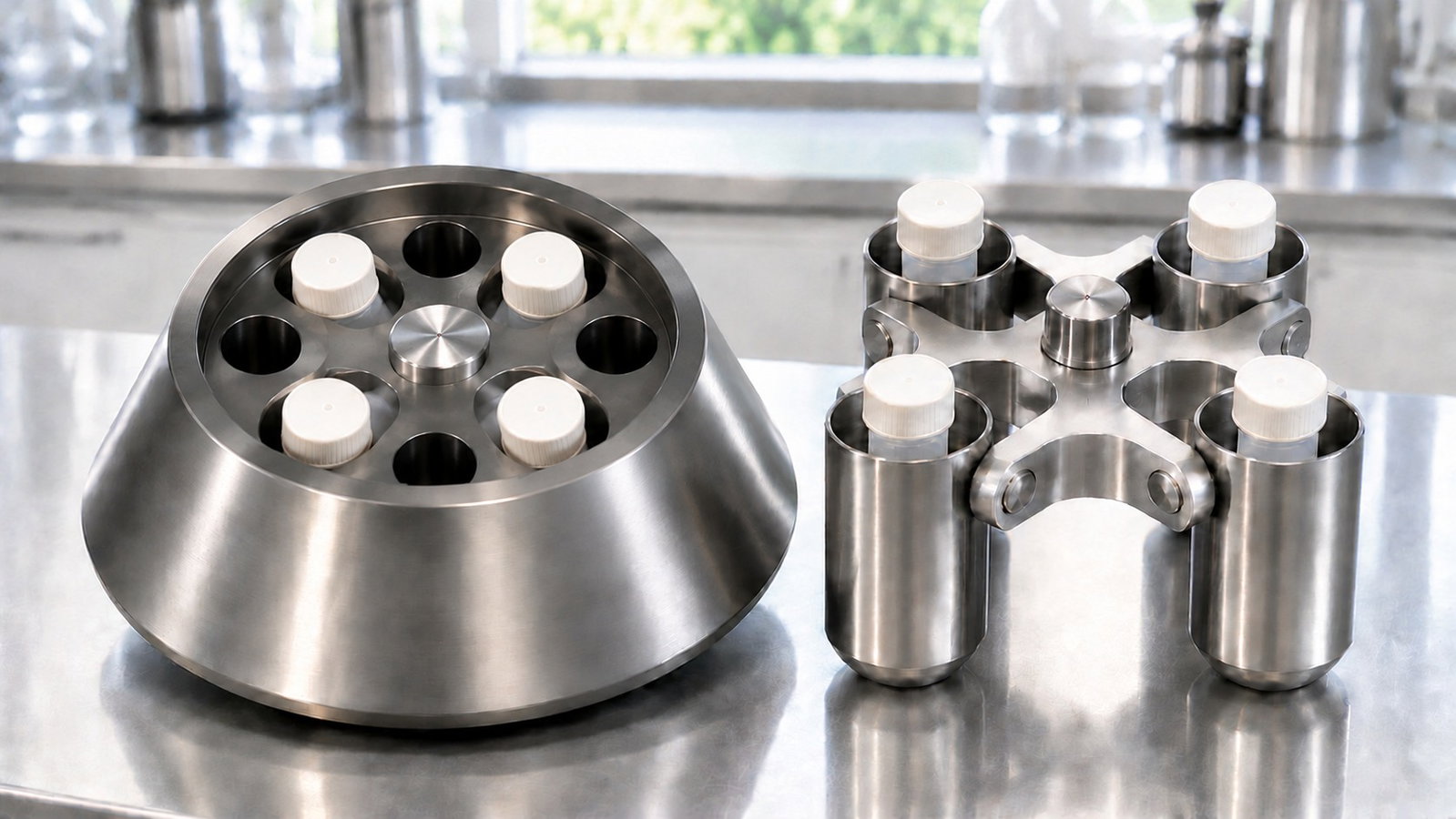
1. Two Geometries, One Physics
RCF is centrifugal acceleration at a specified radius divided by standard gravity: RCF = 1.118 × 10⁻⁵ × r × N², with r in centimeters and N in rpm. Particle motion relative to the liquid also depends on buoyancy, drag, diffusion and fluid motion [1][2][6]. The outward-migration examples below assume a positive sedimentation coefficient; rotation does not make every particle move outward or establish where a recoverable pellet forms.
Fixed-angle rotors hold tube axes at a specified, constant angle to the rotation axis. No numerical angle is assigned to an ACS rotor here. At steady rotation, neglecting capillarity, a free liquid surface is normal to the resultant of gravity and centrifugal acceleration and is generally curved [7]. When centrifugal acceleration dominates, a small local patch can be nearly parallel to the spin axis; that is an approximation, not an exact plane throughout a run.
Swing-bucket rotors (also called swinging-bucket or swing-out rotors) use pivoted carriers whose orientation changes with speed. In the horizontal-running idealization, the tube axis is approximately radial at operating speed and the carrier returns toward its rest position during stopping. The angle during transitions and the actual operating position depend on the design. These are generic principles, not classifications inferred from ACS part names or the word "bucket."
Vertical and near-vertical rotors, ultracentrifuge operation and density-gradient procedures are outside this guide.
| Tube held at a fixed angle | Horizontal-running swing-bucket idealization | |
|---|---|---|
| Tube orientation | Specified tilt to the rotation axis | Carrier angle changes; tube axis approximately radial at speed |
| Outward migration | May encounter the outer side wall before the distal end | A particle near the inner boundary may traverse much of the radial column |
| Distance requiring definition | Distance to first wall contact is not necessarily the complete collection path | Column span depends on the actual tube, fill and operating position |
| Sediment location | Can include the outer wall and distal region | Can collect near the distal tube end |
| Interfaces during transitions | Can reorient and be disturbed | Also change orientation; flatness and preservation are not guaranteed |
The table compares idealized geometry, not product ratings or measured recovery. Use the documented limits of the complete centrifuge, rotor, tube and adapter configuration.
2. Path Length: How Far a Particle Has to Travel
For an outward-sedimenting particle, the starting position, local velocity and collection boundary all affect the travel time. First contact with a wall, clearing the supernatant and forming a recoverable compact pellet are different endpoints. A geometric distance alone does not determine which endpoint has been reached.
In an angled tube, consider a local two-dimensional model with parallel radial trajectories and a straight cylindrical bore of diameter d. If its axis lies in the radial-axial plane at angle θ to the spin axis, a full-bore radial crossing satisfies L cos θ = d, hence L = d/cos θ. An assumed 15 mm bore gives 16.0, 17.3 and 21.2 mm at 20°, 30° and 45°. These calculated chords require the trajectory to intersect both side walls; the meniscus, finite tube ends and actual starting point can truncate them. They are not complete pelleting paths. Boycott's original observation concerned faster gravitational settling in inclined vessels [3]. Later experiments describe a clear-liquid upflow and suspension circulation [5]; this is more than individual particles sliding down a wall and supplies no universal centrifuge-time correction.
In a radially aligned tube, an outward-moving particle starting near the inner liquid boundary may need to traverse most of the column to reach the distal end. A chosen 90 mm column illustrates a longer distance than the chords above; it is not a dimension inferred from a nominal 15 mL tube. RCF changes with radius, and wall contact is a different endpoint, so the distance ratio alone is not a clearing-time ratio.
A higher maximum RCF need not give a shorter modeled transit time. Reducing fill can also change the relevant radial span, but the relationship between volume, surface position and wall-interception path depends on geometry. Do not infer a fill-to-radius mapping or underfill a tube outside its specified operating requirements.
3. Force Is Not Constant Down the Tube
At a fixed speed, two points at radii r_1 and r_2 have RCF_1/RCF_2 = r_1/r_2. Thus a point at half another point's radius has half its RCF. In the radial-column model below, r_min and r_max are defined starting and collection endpoints. The liquid surface and physical tube bottom cannot universally be assigned those roles in an angled or partly filled tube.
That is why the radius at which a figure is quoted matters, and why it changes with the tube and adapter. The specified radii of two ALab™ centrifuges show this directly, independent of any rotor geometry:
- DM0412: the A12-10P rotor is specified at 11 cm and 2,490 ×g at 4,500 rpm for tubes seated directly, and at 9.8 cm and 2,218 ×g for shorter tubes carried in the A10P15 adapter with a plug. Same rotor and speed, about 11 % less force, because the tube sits closer to the axis (DM0412 Low-Speed Centrifuge).
- DG1616 / DG1616R: for the SE4-100 rotor, a four-bucket rotor with tube configurations that vary by bucket set, the specified radius at 4,000 rpm ranges from 14 cm and 2,500 ×g (13 × 75 mm tubes with a plug) to 16.5 cm and 2,950 ×g (13 × 100 mm tubes) (DG1616 / DG1616R High-Speed Centrifuges).
These are the specified RCF reference radii and ratings, not measurements of a complete sedimentation path. Their reference point and inner endpoints are not specified. Confirm the exact tube/adapter/plug mapping. One applicable radius supports RCF at that point; it does not identify geometry or supply a model-specific k-factor. No ACS k-factor or pelleting time is calculated here.
4. The k-Factor (Clearing Factor)
The conventional k-factor expresses a defined radial migration model in convenient units. Its value combines two radial endpoints and a speed; it is not a universal recovery-efficiency measurement. For real labware, check how the supplier defines those endpoints and the associated fill and speed [4].
For the ideal calculation, let σ = (dr/dt)/(ω²r) be a positive, constant sedimentation coefficient in seconds, with angular speed ω in radians per second. Let s denote its numerical value in Svedbergs: σ = s × 10⁻¹³ seconds. Assume constant speed, negligible diffusion and convection, and an unobstructed radial trajectory from r_min to r_max [6, Eqs. 1–4]. Integration gives:
t_seconds = ln(r_max/r_min) / (σ × ω²).
With ω = 2πN/60 and time in hours, the conventional numerical form is [4]:
- k = 2.533 × 10¹¹ × ln(r_max/r_min) / N², with N in rpm.
- t(hours) = k/s, with s the numerical sedimentation coefficient in Svedbergs.
Use natural logarithms and the same length unit for both radii. The rounded coefficient is (10¹³/3600) × (60/2π)². The model time describes reaching the specified endpoint, not pellet compaction, retained recovery or a complete machine cycle.
Four properties follow directly, and they are what make k useful.
Lower k gives a shorter ideal time at unchanged s. In this model, k = 1,000 gives half the transit time of k = 2,000 for the same positive s. This is not a geometry-wide ranking or an observed recovery result.
k scales inversely with speed squared when the endpoints are unchanged. If a specified k refers to speed N_ref, k_adj = k_ref × (N_ref/N_actual)². Confirm the reference speed, fill and endpoint convention rather than assuming full tubes at maximum speed. Halving speed quadruples this model's k and, at unchanged s, its transit time.
k depends on the ratio of radii, not their difference. A rotor whose liquid column starts close to the axis has a large r_max / r_min ratio and a high k, even if its maximum RCF is impressive. This is the quantitative form of the path-length argument: long columns that start near the axis are slow to clear.
A k-ratio gives a conditional time ratio. At the same applicable s and equivalent model endpoints, t_2 = t_1 × k_2/k_1. Calculate each k for the actual speed and defined fill. Sample, medium, temperature, concentration, wall interactions and run profile require separate assessment. Scaling a protocol's recorded duration does not establish that its original endpoint was k-limited or that the new method is equivalent.
5. Worked Example: Two Hypothetical Rotors
Hypothetical rotors A and B below are radius-endpoint models at 4,000 rpm, not commercial hardware. No tube angle, bore, nominal volume or physically validated rotor layout is assigned. The assumed particle has constant s = 10,000 S solely for arithmetic. The table does not establish a fixed-angle versus swing-bucket performance ranking.
| Hypothetical rotor endpoint model | r_min (cm) | r_max (cm) | Radial span r_max - r_min (cm) | RCF at r_min (×g) | RCF at r_max (×g) | k at 4,000 rpm | Model time for s = 10,000 S |
|---|---|---|---|---|---|---|---|
| A: assumed radial endpoints | 7.0 | 14.0 | 7.0 | 1,252 | 2,504 | 10,973 | ≈ 66 min |
| B: assumed radial endpoints | 6.0 | 16.0 | 10.0 | 1,073 | 2,862 | 15,528 | ≈ 93 min |
B has about 14.3% higher maximum RCF but a 41.5% larger k, so its ideal endpoint time at the assumed s is longer. That follows from the chosen radii, not an assigned rotor type. Separately, the ratio calculation maps 10 minutes in B to about 7.1 minutes in A (10 × 10,973/15,528). Neither duration is the table's full-transit estimate for s = 10,000 S: those are about 93 and 66 minutes. The ratio example does not establish complete pelleting or an equivalent experimental endpoint.
Two further changes show how sensitive k is to operating conditions:
- Lower speed. Running rotor A at 3,000 rpm instead of 4,000 rpm raises k to 10,973 × (4,000 / 3,000)² ≈ 19,500, and the estimated time for the same particle from about 66 to about 117 minutes.
- Changed starting radius. Assume r_min moves from 7.0 to 10.5 cm while r_max stays 14.0 cm. At 4,000 rpm, k becomes about 4,550 and the model time about 27 minutes. These are chosen endpoints, not a derived half-volume fill: that mapping requires tube geometry and the rotating liquid configuration. Check permitted fill and support requirements before considering a real volume change.
Using maximum RCF × time instead gives 10 × 2,862/2,504 ≈ 11.4 minutes in A, rather than the 7.1-minute k-ratio result. The two calculations preserve different quantities. Neither the maximum-RCF product nor similar-looking geometry establishes equivalent separation. The comparison is algebra, not a recommendation to choose either duration for an experiment.
6. Pelleting Time in Practice: Where k Stops Being Exact
The k-factor is a model, and its assumptions matter as soon as you rely on the number.
- Ideal migration. The derivation assumes an independent, nondiffusing particle with constant positive s, constant speed and an unobstructed radial path. It does not model startup from rest, sediment compaction, aggregation, convection or concentration-dependent interactions [6].
- Applicable s. Use a coefficient appropriate to the actual medium, temperature and particle state, not an unconverted reference-condition value. Changes in density, viscosity or particle properties can change s; geometry-only k does not make those corrections [1][2][4].
- The collection boundary. In an angled tube, first wall contact and subsequent transport need not match an unobstructed r_min-to-r_max trajectory. Wall adhesion, fluid motion and deposition can change recovery. No universal conservative upper bound on clearing time follows from the formula or from the Boycott effect [3][5].
- The run profile. For the same ideal constant-s particle, changing speed requires the integral of ω(t)² over time [6]. Neither a programmed duration nor a ramp-time number establishes that integral or a validated pelleting endpoint.
- Staying collected. Deceleration and handling can disturb sediment or interfaces. Reaching a model boundary does not establish retained recovery or pellet quality.
Large or irregular particles can have effective sedimentation coefficients under defined conditions, but a heterogeneous preparation may not be represented adequately by one constant s. When the coefficient or model applicability is unknown, the formula supplies no validated time. Define and assess the experimental endpoint rather than assigning a value from the sample category.
7. Pellet Shape, Interfaces and Recovery
Speed of clearing is only half the comparison; what the separated sample looks like at the end of the run is the other half.
Angled tubes can collect material on the outer side wall and toward the distal end, depending on tube shape, fill, sample and handling [1][2]. Wall contact can complicate recovery, but neither a streak nor a bottom pellet is guaranteed. Use the approved tube orientation and recovery procedure; a generic cap-hinge rule does not replace the actual loading instructions. Acceleration and braking can disturb the sample, and a longer stop does not guarantee preserved recovery.
Tubes that approach radial alignment can direct outward sediment toward the distal end and align interfaces across the tube during steady rotation. Pellet compactness and recovery still depend on the sample and conditions. The field and carrier orientation change during acceleration and stopping, so interfaces are not guaranteed to remain flat or undisturbed. Density-gradient procedures and their specialized rotor choices remain outside this guide.
Compare the required endpoint and complete assembly, not a presumed speed-versus-recovery trade-off. Fit, load and balance cups, buckets, lids and adapters exactly as the configuration's instructions require; neither geometry name supplies an approved installation or partial-load pattern.
8. When Each Geometry Tends to Fit
The table lists geometry-related considerations, not universal task recommendations. The approved method and complete configuration determine the choice.
| Task | Geometry consideration | What must be checked |
|---|---|---|
| Rapid pelleting | An angled tube may shorten travel to a wall | Applicable k or model, actual collection boundary and measured recovery |
| Microtubes at high RCF | Neither geometry name establishes a speed rating | Approved rotor/tube/adapter rating and required endpoint |
| Recovering a bottom pellet | Radial alignment may favor distal-end collection | Pellet location, compactness and the recovery method |
| Preserving a liquid interface | Orientation at speed matters, but transitions can disturb either design | Complete speed profile, fill and post-run handling |
| Microplates or deep-well plates | Use a documented compatible carrier | Orientation, plate support, stacking and loading limits |
| Large volumes | Capacity is a configuration property, not a geometry guarantee | Listed vessels, adapters, mass limits and ratings |
| Repeated solid washing | Either design may be considered | Retained yield, redispersion and cumulative losses |
Geometry never permits exceeding instrument, rotor, tube, adapter or load limits. For a method change, define recovery, purity, interface or other acceptance criteria and assess the complete configuration. A recalculated time alone is not approval of the transfer.
9. Reading a Rotor Table Before You Compare
To compare rotors on pelleting performance rather than headline force, you need more than maximum rpm and maximum RCF. For each rotor and tube or adapter configuration, ask for:
- Documented geometry and operating angle. Do not infer them from a name, an A- or AS-prefixed code, the word "bucket" or a photograph.
- Defined radial endpoints for the actual tube, adapter and permitted fill, identifying whether they describe first wall contact or another collection boundary.
- A documented k-factor and its basis: speed, fill, endpoint convention and applicable model, rather than an assumed full-tube value.
- Permitted speed and RCF for the complete configuration, including tube/adapter effects and reference-radius definition.
- Operating and recovery requirements: loading, closures, sample conditions, run profile and endpoint verification.
As neutral specification context, the DG1616 / DG1616R has eleven listed rotors. SR4-200 and SR4-400 are associated with "hanging cups, lids and handles" and adapter options; SE4-100 has four buckets, with tube configurations that vary by bucket set. Specified SR4-200 values are 5,500 rpm / 5,495 ×g / 16.25 cm; SR4-400 values are 5,000 rpm / 4,639 ×g / 16.6 cm. The SE4-100 radii are specified by bucket set. These are ratings, not geometry labels or k inputs: the radius definition, inner endpoint, operating angle and k-factor are not specified. No rotor on it is identified here as fixed-angle or swing-bucket.
The same applies to every rotor you consider: if the geometry or the radius span is not specified, ask before relying on a time conversion.
10. Converting a Method Between Rotors
When a protocol was written for one rotor and you need to run it on another, work through these steps.
- Identify the original configuration and endpoint: instrument, rotor, tube/adapter, fill, sample, medium, temperature, speed history, timing convention and recovery requirement.
- Check both model definitions. Obtain applicable k values or justified endpoints for the actual speeds and fills. Do not substitute an undefined single radius.
- Use a ratio only when justified. At unchanged applicable s, t_new = t_old × k_new/k_old is a conditional model estimate, not a validated protocol setting.
- Check all assembly limits. Confirm permitted speed, RCF, fill, loading and other requirements before any method-development run.
- Assess the defined endpoint. Use an approved transfer plan with appropriate measurements and repeatability checks; visual pellet similarity or one pilot run is not sufficient by itself.
- Record evidence and unresolved fields, including k definitions, assumptions and the acceptance criteria used.
If the geometry, endpoints or applicability are unresolved, no k-based conversion is established. Retaining nominal ×g and time may be considered only within an approved method-development plan, not as a universal fallback. Resolve the evidence gaps rather than reporting a converted time with false precision.
11. Frequently Asked Questions
What is the main difference between a fixed angle and a swing bucket rotor?
A fixed-angle design holds tube axes at a specified constant tilt; a swing-bucket design changes carrier orientation with speed. These change wall-interception paths and potential collection locations, but do not alone determine pellet quality or separation performance. No ACS rotor is assigned either geometry here.
Which pellets faster?
Geometry alone does not decide. At the same applicable s, a smaller k gives a shorter time in the stated migration model. Compare justified endpoints, speed, fill and experimental recovery rather than assuming that every angled rotor is faster.
What is a good k-factor?
There is no universal target. Compare values with documented endpoint, speed and fill conventions. A smaller value reduces the ideal time at unchanged s; it does not by itself establish sample recovery, compatibility or a safe run setting.
Can I calculate a k-factor from a specified radius?
Not from one undefined radius. The radial model needs two justified endpoints and speed, while a supplier's k also needs its tube/fill convention. An applicable specified radius supports RCF at that point, not an inferred geometry or validated clearing time.
If I keep the same ×g and time, will a different rotor give the same result?
Not necessarily, even with similar geometry. Confirm the radius basis, sample and medium, fill, temperature, speed history and recovery conditions. A justified k-ratio can inform a transfer assessment but cannot establish equivalence on its own.
Is a swing-bucket rotor gentler on cells?
No general gentleness or viability advantage is established by the geometry label. The sample, medium, force history, tube contacts, temperature and recovery procedure all require assessment against the method's endpoint.
12. Keep Exploring Centrifugation
- Laboratory Centrifugation: RCF, Rotors, Sedimentation and How to Choose a Centrifuge: the centrifugation hub covering RCF, rotors, sedimentation, temperature, safety and the full series of guides.
Rotor tables with specified radii: DG1616 / DG1616R High-Speed Centrifuges (listed rotors and SE4-100 bucket sets; radius definition not specified) and DM0412 Low-Speed Centrifuge (A12-10P direct seating versus A10P15 adapter and plug).
Browse all ALab™ centrifuges.