
Ask any thermal laboratory how bulk thermal diffusivity gets measured and the answer is almost always the same: laser flash analysis. Since its invention in 1961, the flash method has become the reference technique for disc-shaped bulk samples — standardized, automated, and installed in thousands of laboratories12. That dominance is earned, and this article explains exactly how the measurement works and why it wins on its home ground. But every dominant method has a boundary, and LFA’s boundary is drawn by sample geometry: fibers, films, wires, coatings and micro-samples sit on the far side of it for reasons that are physical, not incidental. Knowing precisely where that line runs — and what takes over beyond it — is the difference between choosing a method and inheriting one.
- 1How the flash method works
- 2The corrections that made it a standard
- 3What LFA measures well — and why it dominates
- 4Where LFA fails: six sample classes
- 5Interactive: extract the half-rise time yourself
- 6LFA against the transient alternatives
- 7Choosing between LFA and suspended-sample methods
- 8Frequently asked questions
- 9Keep exploring the knowledge hub
- 10References
How the flash method works
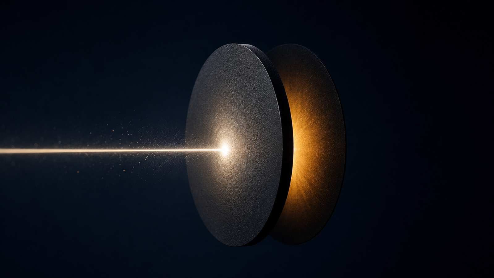
The 1961 paper by Parker, Jenkins, Butler and Abbott is a model of experimental economy1. Deposit a short burst of energy uniformly on the front face of a thermally insulated disc, and one-dimensional conduction carries the heat toward the rear face. The rear-face temperature rise, normalized to its maximum, follows a universal curve — a Fourier series in the Fourier number Fo = αt/L², the natural dimensionless clock of diffusion. Every material traces the same normalized curve; only the time axis stretches, and the half-rise always lands at Fo½ ≈ 0.1388. Reading a single feature of that curve — the moment it crosses half of its final rise — therefore pins the diffusivity, and Parker’s dimensionless constant 0.1388 — the value carried into ASTM E1461 practice — converts the reading into α.
The elegance runs deeper than the formula. Because the method reads a shape rather than an absolute temperature, it does not require absolute thermometry of the rear face — a detector watching relative radiance suffices, provided the response stays linear and the surface emissivity stays stable over the transient. Because the pulse is optical and the readout is optical, nothing touches the sample: no contact resistance corrupts the signal path, a systematic that plagues contact-based techniques3. And because the heat pulse is small and brief, the measurement perturbs the sample only slightly from its furnace temperature, so a single specimen can be walked across a wide temperature program — room temperature to well above 1000 °C in commercial instruments — producing α(T) in an afternoon2.
What LFA returns natively is diffusivity, not conductivity. The conversion k = α ρ cp requires the density and specific heat from separate measurements or a calibrated comparative procedure, and the uncertainty of those inputs propagates into k in full4 — a bookkeeping obligation the technique shares with every diffusivity-first method, including the suspended-sample family this site documents5.
The corrections that made it a standard
Parker’s formula assumes three idealizations: an instantaneous pulse, an adiabatic disc, and uniform absorption on the front face. Real experiments violate all three, and the sixty-year history of LFA is largely the history of correcting them honestly.
The finite-pulse problem came first. If the flash lasts a non-negligible fraction of the diffusion time — routine for thin, high-diffusivity discs — the rear face starts rising before the pulse ends, the apparent half-rise time stretches, and uncorrected analysis reports a diffusivity that is too low. Cape and Lehman’s 1963 analysis treated the finite pulse and, in the same paper, the radiative heat losses that violate the adiabatic assumption at high temperature6. Heat loss pulls in the opposite direction: energy leaking from the faces and rim makes the rear-face curve peak early and sag, shortening the apparent t½ and biasing α high. Two opposing systematics, both invisible in a single reading — exactly the situation where model-based correction, not optimism, is the only defensible path. Modern practice bakes these corrections into the standard: ASTM E1461 prescribes the specimen proportions, pulse characterization and loss models under which flash results are considered defensible2.
The third idealization — uniform absorption — is handled in the sample preparation room rather than the mathematics: translucent or reflective specimens receive a thin graphite coating so the pulse deposits where the model assumes it does. On a thick, moderate-diffusivity disc the coating is a minor perturbation; on thin, fast discs its heat capacity and finite response begin to matter — and on anything micrometers thick it is a first-order problem.
What LFA measures well — and why it dominates
On its home ground the technique is close to unbeatable. The home ground is specific: self-supporting discs, typically (in representative commercial instruments) 6–25 mm in diameter and 1–4 mm thick, of homogeneous, opaque, isotropic material. Ceramics, metals, graphites, dense polymers, sintered thermoelectrics, nuclear fuel surrogates — cut the disc, coat it, load the carousel. Throughput is high, operator skill demands are modest, furnace integration reaches extreme temperatures, and six decades of round-robin validation stand behind the number26.
It is worth being explicit about why the wins are structural. The measurement needs no fabricated heater or sensor on the sample — so there is no lithography, no sputtering, no contact-resistance audit3. Because the rise curve is normalized, absolute detector calibration largely cancels when detector response is linear and surface emissivity remains stable over the transient. And the disc geometry gives the heat pulse a large, well-defined one-dimensional stage. Every one of those advantages, note, is purchased by the disc itself: a sample massive enough to machine, opaque enough to coat, and thick enough that its front and rear faces are distinct thermal events.
Where LFA fails: six sample classes
Each failure below is physical — a place where the disc-shaped, rear-face-radiance architecture stops being a measurement and starts being an assumption.
1. Fibers, wires and filaments. A carbon fiber, a metallic microwire, a spun graphene fiber7 cannot be made into a disc, and a bundle pressed into one measures the bundle’s contact network, not the filament8. Axial transport in a single suspended filament is the property engineering actually needs — and it is exactly the geometry the flash architecture cannot address.
2. Thin films in-plane. Flash through the thickness of a micrometer film would need nanosecond-resolved rear-face thermometry on a sample that barely absorbs the pulse; flash along the film is not a defined experiment. In-plane transport of films and membranes belongs to electrothermal and thermoreflectance families built for it910.
3. Micro-samples. Below a few millimeters of lateral extent, the deposited pulse energy and the rear-face radiance both collapse, and the finite-pulse correction swallows the signal it was meant to refine6. Suspended micro-bridge devices11 and transient electro-thermal platforms5 were invented precisely because the flash architecture runs out of photons here.
4. Coatings and layered stacks. A flash result on a coated disc is a composite number; decomposing it requires a multilayer inversion in which the interface conductance joins the unknowns — feasible in principle, but with parameter correlation and identifiability doing real damage in practice3. Layer-resolving techniques such as time-domain thermoreflectance were developed to make that decomposition an explicit, sensitivity-audited fit rather than an assumption1012.
5. Strongly anisotropic materials. A through-thickness flash on a rolled graphite or aligned composite reads the cross-plane value only; the in-plane number — often ten to a hundred times larger — requires special radial configurations or a different method family altogether13. Reporting one axis of an anisotropic tensor as “the” conductivity is a datasheet failure mode our claim-validation article dissects.
6. Translucent and low-emissivity specimens at the micro scale. The graphite-coating fix that is benign on a bulk disc becomes a competing thermal layer on anything thin: on a micrometer sample the coating’s own heat capacity and conductance enter the measurement at first order — the exact composite-correction problem the suspended-sample coating protocol treats explicitly14.
None of this is a defect of LFA; it is the price of its architecture. The honest summary: the flash method owns the bulk disc, and delegates everything the disc cannot represent.
Interactive: extract the half-rise time yourself
The simulator below draws the normalized rear-face temperature rise and lets you corrupt it the two ways real experiments do. Stretch the pulse width and watch the apparent half-rise time inflate — uncorrected α drops. Add face heat losses and watch the curve peak early and sag — uncorrected α climbs. The two biases run in opposite directions, which is exactly why a laboratory cannot wave at them qualitatively: the correction models62 exist because the raw reading, alone, cannot tell you which way it is wrong.
LFA against the transient alternatives
| Method | Native sample form | Measured quantity | Contact with sample | Characteristic strength | Characteristic limit |
|---|---|---|---|---|---|
| Laser flash (LFA)12 | Self-supporting disc, mm thickness | Through-thickness α | None (optical in, optical out) | Bulk standard; extreme-temperature furnaces; throughput | No fibers, films, micro-samples; composite numbers on stacks |
| Transient plane source (Hot Disk)15 | Two solid halves clamping a sensor | k and α of bulk isotropic solids | Sensor pressed between halves | Minimal preparation; wide k range16 | Contact quality; probing-depth window discipline |
| 3ω9 | Film or bulk under a fabricated metal line | Cross-plane k of films, bulk k | Lithographed heater line | Sub-micron films; rigorous frequency-domain model | Fabrication per sample; electrically insulating surface needed |
| TDTR1012 | Polished surface with metal transducer | k of films, interface conductance G | Sputtered transducer film | Interface sensitivity and parameter identifiability3 | Parameter correlation between k and G; instrument cost |
| Suspended micro-bridge11 | Nanostructure placed across two membranes | Thermal conductance of 1D nano-objects | Sample bridges fabricated device | Single nanotubes and nanowires17 | Device fabrication; contact thermal resistance budget |
| Transient electro-thermal (TET)518 | Suspended fiber, wire or film strip | Axial α (k, ρcp with companions) | Silver-paste mounting at two electrodes | The fiber/film/micro geometry LFA cannot hold; validated few-percent protocols (under the stated specimen and correction conditions)19 | Sample must carry (or be coated to carry) a sensing current14 |
Choosing between LFA and suspended-sample methods
The decision is geometric before it is anything else. If the sample can honestly become a millimeter disc — homogeneous, opaque, isotropic — LFA is the default, and arguing with six decades of standardization is a poor use of a laboratory’s time2. If the sample is a fiber, a wire, a film strip, a micro-scale specimen or a coated architecture, the disc never existed to begin with, and the suspended-sample electrothermal family — TET and its accuracy-oriented extensions documented across this knowledge hub — is the geometry-native path51820. Between the two sits the honest gray zone: bulk anisotropy, layered stacks, and samples that could be forced into a disc at the cost of measuring the wrong thing. For those, the method-selection framework in the companion pillar article — and, where the stakes justify it, a specimen-specific feasibility review with our thermal testing team — beats any one-line rule.
One quantitative anchor for the boundary: uncertainty budgets. A well-run flash measurement on a conforming disc carries a few percent uncertainty in α2; a well-run suspended-fiber TET campaign, with the zero-rise and differential protocols applied, operates in the same few-percent territory on samples LFA cannot hold at all1418. The choice, in other words, is not between an accurate method and a compromise — it is between two accurate methods with disjoint geometric jurisdictions, plus the statistical machinery both share2122.
Frequently asked questions
Can laser flash analysis measure thin films?
Not in the film regimes that dominate modern questions. Through-thickness flash on micrometer films would demand pulse and detection timescales far beyond the standard architecture, and in-plane film transport is outside the flash geometry entirely. Film work belongs to 3ω9, TDTR10 and, for free-standing strips and membranes, the suspended electrothermal family5.
Why does my sample need a graphite coating for LFA?
Two jobs at once: the coating absorbs the pulse on a reflective or translucent front face, and it fixes the rear-face emissivity so the infrared detector sees a clean radiance signal. On a sufficiently thick, moderate-diffusivity disc the coating is often a small perturbation under validated conditions; on anything thin it becomes a real layer in the measurement — one reason micro-scale samples exit the flash architecture14.
Is TET more accurate than LFA?
Wrong axis of comparison. On a conforming bulk disc, standardized LFA is the reference and there is no reason to displace it2. On fibers, films and micro-samples the disc does not exist, so the comparison is between TET’s few-percent validated protocols19 and no measurement at all. Jurisdiction first, accuracy second.
Keep Exploring the ACS Thermal Metrology Knowledge Hub
This article is one chapter of the ACS thermal metrology knowledge hub. To keep going:
- Thermal conductivity & diffusivity testing: the pillar guide — methods, samples and a buyer’s framework in one place.
- Which thermal measurement method should you use? — the interactive decision hub this article feeds into.
- The TET technique: a complete guide — the suspended-sample method that takes over where the disc ends.
- Differential TET — how suspended-sample work audits its own parasitics.
- Thermal testing services — send us the sample; get defensible numbers back.
References
This article describes laser flash analysis and its comparison with transient electro-thermal and related methods for educational purposes. Idealized formulas and the interactive model are schematic teaching tools; real measurements follow the applicable standards, correction models and instrument documentation. For sample-specific feasibility, datasheets and SDS, contact our thermal testing team.