The Transient Electro-Thermal (TET) Technique: A Complete Guide

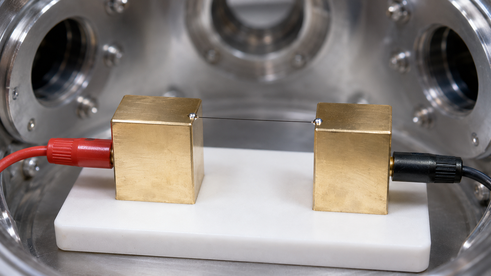
A fiber thinner than a human hair is suspended across two electrodes inside a small vacuum chamber. A modest direct current switches on; over the next fraction of a second the voltage across the fiber drifts by a few millivolts and settles. That is the entire experiment — and inside that short transient sits the fiber’s thermal diffusivity, extracted through a closed-form solution of the heat equation. This is the transient electro-thermal (TET) technique: no lithographically patterned heater lines, no microfabricated measurement platform — though electrically non-conductive samples do take a thin characterized metallic coating. The sample is the sensor. This guide walks through how a TET measurement works end to end — the physical idea, the setup, the governing solution, the signal chain, and where the method sits among its alternatives.

The idea: the sample is the sensor

Most microscale thermal measurements split the job in two: something injects heat (a laser, a fabricated heater line) and something else reads temperature (a deposited thermometer, an optical probe, a radiation detector). Each added element brings its own calibration, its own interface and its own uncertainty budget. The TET technique collapses the two roles into the sample itself². A step direct current through a suspended conductor generates distributed Joule heating along its length; the same conductor’s electrical resistance changes with temperature, so the voltage across it tracks the evolving average temperature in real time. One current source, one voltmeter, one sample — and the physics of one-dimensional transient conduction does the rest.

The elegance is not merely aesthetic. Because electrical heating is distributed along the suspended gauge length and resistance sensing is spatially averaged over that same gauge length, the method avoids assigning the response to a single optical spot or point-thermometer coupling — for coated nonconductive specimens, the coating–sample thermal coupling and the coating’s own conductance must be included in the validated model — a class of assumptions that can complicate optical-probe methods. What it does require is a sample that carries current (directly, or through a thin metallic coating), a well-defined suspended length, and boundary conditions clean enough for the one-dimensional model to hold.

Anatomy of a measurement

A TET measurement has four working parts. (1) The suspended sample. A wire, fiber or narrow film strip is mounted across a gap between two massive electrodes — typically with silver paste or conductive epoxy at the contacts — so that the suspended length is defined and the ends are held near the electrode temperature during the transient³. (2) The vacuum. The chamber is evacuated — below roughly 0.2 mTorr in our current validated workflow — so that convective heat loss from the sample surface becomes negligible and conduction along the sample dominates; radiation remains and is handled in the analysis or by dedicated corrections for high-emissivity or very thin samples. (3) The current step. A source switches from zero to a constant current chosen large enough to produce a clean, resolvable voltage change and small enough to keep the temperature rise modest — a balance treated rigorously in the zero-temperature-rise extension of the method. (4) The acquisition chain. A voltage amplifier and digitizer record V(t) from the instant of the step until a steady state is reached, over milliseconds to seconds depending on sample length and diffusivity.

For electrically non-conductive samples — polymer fibers, ceramic filaments, biological fibers — a thin metallic film (commonly gold, tens of nanometers) is coated onto the surface to carry the current. The coating adds a parallel heat path whose contribution must be quantified or removed through a validated differential-coating analysis or model subtraction³ — making the film thin helps, but thinness alone does not establish that its thermal contribution is negligible.

The governing solution

With the two ends held at the sink temperature and spatially distributed electrical heating (under the ideal one-dimensional model) switched on at t = 0, the one-dimensional heat equation for the suspended segment has a classical series solution. Written for the normalized average temperature rise T*(t) — the instantaneous average temperature rise divided by its steady-state value — it takes the form²:

T*(t) = (96/π⁴) Σ_m odd (1/m⁴) [1 − exp(−m²π²αt/L²)]

Two features make this equation a measurement instrument rather than a textbook exercise. First, T*(t) depends on the material through a single grouped parameter, the Fourier number Fo = αt/L²: the sample’s length is measured under a microscope, time is measured by the digitizer, and α is the only unknown. Second, the series converges rapidly: after the short early-time region, the first eigenmode dominates the remaining transient — the companion linearization article quantifies the residual higher-mode contribution and the practical fit-window criteria — which is precisely the property the linear-regression analysis of the next articles in this series exploits. The characteristic thermal time of the experiment scales as L²/α: a few-millimeter carbon fiber settles in tens to hundreds of milliseconds, while a low-diffusivity polymer fiber of the same length can take seconds.

The same solution defines the method’s honest boundaries. It assumes one-dimensional conduction (length much greater than the cross-sectional dimension), end temperatures pinned by the heat sinks, approximately uniform heat generation per unit length along the suspended gauge, and material properties that remain nearly constant over the small imposed temperature rise — for coated nonconductive specimens, the coating–sample thermal coupling and the coating’s own electrical and thermal conductance form part of the validated measurement model. Each assumption is checkable, and the family of extensions discussed below exists largely to relax them one at a time.

From voltage transient to temperature rise

The raw observable is voltage, not temperature. The bridge between them is the sample’s temperature coefficient of resistance: within a modest temperature window, resistance varies linearly with average temperature, so the normalized voltage change reproduces the normalized average temperature rise directly — V(t) rescaled between its initial and steady-state values is T*(t), without requiring the absolute coefficient to be known². This is a quiet but decisive advantage: diffusivity extraction needs only the shape of the transient, not an absolute temperature calibration. The absolute coefficient matters only when the same experiment is extended to deliver thermal conductivity or specific heat as well, which has been demonstrated by combining transient and steady-state information from the same suspended-sample configuration⁴.

Practical signal quality determines everything downstream. The current must be steady during the step; contact resistance at the electrodes must be stable — four-probe configurations remove electrical lead and contact resistance from the measured voltage, though not thermal contact resistance or imperfect end-boundary conditions; and the digitizer must resolve the early transient without distorting it. Nonlinear effects — radiation at elevated temperature, temperature-dependent properties in strongly nonlinear materials — have been characterized within the method and set the boundaries within which the linear analysis holds⁵.

What it measures, and on what

The native output of TET is in-plane (axial) thermal diffusivity. Combined with independently known density and specific heat — or with the extended analysis that extracts heat capacity from the same setup⁴ — it yields thermal conductivity. The sample classes are one-dimensional and quasi-one-dimensional structures: metallic and non-metallic wires, carbon and polymer fibers, biological filaments, and free-standing film strips. In the commercial implementation, our ThermalSure® TEPT X1 characterizes wires from roughly 0.2 μm to 300 μm in diameter and films from roughly 0.5 μm to 300 μm in thickness, over a diffusivity range of about 0.5×10⁻⁷ to 2.0×10⁻³ m²/s — specifications and sample requirements are on the TEPT X1 product page.

The published record of the technique spans an unusually wide materials range: micron-scale conductive and non-conductive wires in the founding work², protein-based fibers whose measured conductivity revealed unexpected structure–property behavior, lignin-based and PAN-based carbon fibers, CVD graphene and graphene fibers, and down to atomic-thickness two-dimensional materials in the modern era — a scope reviewed comprehensively in 2025⁶. A suspended specimen may be in range when its geometry, resistance, temperature coefficient, mechanical stability, end contacts and expected transient time all fall within a validated measurement window — suspendability and conductivity alone do not establish feasibility; if you are unsure, this is exactly the question our thermal testing service answers before any measurement is quoted.

Three examples from the published record convey the range concretely. Spider silk, measured by this family of methods, revealed exceptionally high thermal conductivity for a protein fiber and an abnormal increase under stretching — a discovery about a biological material possible without a microfabricated suspended platform or lithographically patterned heater — though a characterized conductive coating and stable end contacts were still required⁷. A single carbon fibre, measured along its axis, showed how thermal diffusivity tracks internal structure — turning the measurement into a structural probe⁸. And lignocellulose fibers have been characterized down to 41 K, demonstrating that the same suspended-sample concept extends across a wide cryogenic-to-ambient window when the cell-scale structure demands it⁹. Conductive metal, structural carbon, biological protein and plant matter — one measurement idea spans them all.

Related suspended-sample electrothermal and photothermal methods

TET sits inside a broader toolkit of suspended-sample electrothermal and photothermal methods, and honest genealogy matters: some are direct variants of TET, others are independent siblings that share the philosophy but not the parentage. Direct variants and extensions of TET include the transient photo-electro-thermal (TPET) route, which replaces electrical heating with a step laser while keeping electrical sensing, decoupling the heating current from the sensing current for delicate samples¹⁰; the coating- and length-differential analyses that isolate parasitic channels; zero-temperature-rise extrapolation; and the linearized-regression reduction treated later in this series. Related but distinct methods stand on their own: the optical-heating electrical-thermal-sensing (OHETS) approach, published in 2006 — before TET — applies harmonic optical heating with electrical sensing to conductive and non-conductive wires alike¹¹; pulsed laser-assisted thermal relaxation (PLTR) reads the free cooling decay after a laser pulse rather than a heating rise¹²; a steady-state electro-Raman-thermal route trades transient acquisition for Raman thermometry of the electrically heated sample¹³; the Johnson-noise electro-thermal variant reads temperature from thermal noise, removing the temperature-coefficient requirement¹⁴; and a separate differential thermal resistance method reaches microscale sample lengths by differencing configurations¹⁵. Later articles treat the data-analysis branches — characteristic-point, global fitting and the patented linear-regression route; the full map lives in the pillar guide.

What can go wrong — and how the method answers

An honest guide names the failure modes. Contact quality comes first: a soft or drifting electrode joint distorts both the electrical signal and the thermal boundary condition; the answer is rigid mounting, conductive adhesive cured properly, and four-probe sensing that removes electrical contact resistance from the measured voltage³. Radiation is second: a thin sample with appreciable emissivity loses heat from its surface in parallel with axial conduction, inflating the apparent diffusivity; the family’s differential analyses measure across systematically varied lengths or coatings and extrapolate the surface channel away³. Coating influence is third for non-conductive samples: the metallic film that carries the current is itself a parallel heat path, whose contribution must be characterized — thickness, continuity, electrical and thermal conductance — and removed through the dedicated coating model or differential extrapolation in the published experimental protocol; thinness reduces the term but does not by itself establish negligibility³. Nonlinearity is fourth: strongly temperature-dependent properties bend the assumptions of the linear model, a regime that has been explicitly characterized so its onset is known rather than guessed⁵. None of these is exotic; all are routine checklist items in a disciplined measurement — and many of them leave detectable signatures in the transient or its residuals if you look — while others require differential measurements, reference specimens or independent boundary checks — which is still an underrated virtue of a method whose entire signal is one honest curve.

TET among the alternatives

No single method owns microscale thermal metrology, and honest selection is geometry-driven. The 3ω method excels for thin films on substrates and for samples where a metal line can be fabricated, extracting properties from the third-harmonic response of an AC-heated line¹⁶ — but it requires that fabrication step. Laser flash is the industrial standard for bulk slabs and disks, timing a heat pulse through the thickness¹⁷ — but it needs a planar specimen large enough to mount and assumes through-thickness one-dimensionality. Time-domain thermoreflectance is highly effective for thin films, multilayers and interfaces, with depth- and parameter-sensitivity set by modulation frequency, transducer properties, beam size and the multilayer model¹⁸ — formidable capability, purchased with optical complexity and model dependence. TET occupies a niche these alternatives often serve less directly: free-standing one-dimensional samples — the wire you can hold, the fiber you spun, the film strip you peeled — measured whole, without microfabrication — and once a specimen is mounted, contacted and the chamber prepared, the transient acquisition itself is rapid. Choosing among them is a geometry-and-question decision, which is why our testing service leads with sample form, not with a default method.

The next article in this series takes the V–t curve this technique produces and asks the deceptively simple question: how exactly do you turn it into a number — and why do different reduction routes give different answers? Continue to TET data reduction.

Keep Exploring the ACS Thermal Metrology Knowledge Hub

This article is one chapter of the ACS thermal metrology knowledge hub. To keep going:

• Thermal conductivity & diffusivity testing: the pillar guide — methods, samples and a buyer’s framework in one place.
• From V–t curve to diffusivity — the three data-reduction routes compared.
• Linearized TET regression — fit stability and regression-level uncertainty.
• TPET: laser-heated characterization — decoupled optical heating with electrical sensing.
• Zero-temperature-rise extrapolation — removing self-heating bias, validated on a Pt wire.
• ThermalSure® TEPT X1 — the instrument implementing this measurement family.

This guide describes the transient electro-thermal technique as implemented for free-standing wires, fibers and films. Governing equations are presented in their idealized one-dimensional form; real measurements include boundary, radiation and coating considerations addressed in the companion articles and in method documentation. Performance figures for specific instruments refer to their published specifications. The interactive simulator is a schematic teaching tool, not a substitute for measurement.