
Hand the same voltage transient to three careful analysts and you can get three different thermal diffusivities — not because anyone blundered, but because the curve can be reduced through several commonly encountered routes — not all equally defensible over the same part of the transient — each with its own sensitivity to noise, truncation and model mismatch. This article walks through three instructive reduction routes commonly encountered in TET analysis, shows where each one is strong, where each one quietly fails, and why the differences between them are not pedantry: they are exactly the kind of methodological spread that shows up when the same physical sample is measured across methods and laboratories.
One curve, three answers
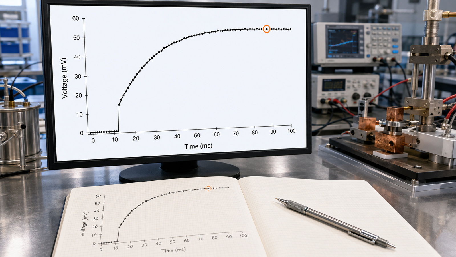
The physics fixes the curve. With both ends of the suspended sample held at the sink temperature and step Joule heating switched on, the normalized average temperature rise follows the series solution T*(t) = (96/π⁴) Σm odd (1/m⁴)[1 − exp(−m²π²Fo)], where Fo = αt/L² is the only material-dependent group2. Every reduction route is an attempt to invert this one relation. What differs is which part of the curve each route trusts — and since real data carry noise at the bottom, drift at the top and a finite acquisition window in between, that choice is consequential.
It is worth being precise about why these three reduction strategies are worth comparing at all, because the reason is structural rather than historical: they weight different portions of the transient differently. The governing relation is nonlinear in Fo, monotonic, and saturating: information about α is not distributed evenly along it. The early rise is information-dense but contaminated by higher modes and instrumentation; the mid-curve balances signal change against mode purity; the late plateau pins the normalization but barely moves with α at all. Any reduction is therefore an implicit weighting of these regions — the single-point routes place all their weight at one location, the global fit spreads it — and the “right” weighting depends on where a particular data set’s pathologies live. Three routes persist because three different pathologies (early contamination, local noise, truncation) each punish a different weighting hardest.
Route 1: the early-time trap
The oldest instinct is to fit the initial rise, where the signal changes fastest. The trap is structural: at early times the series has not collapsed to its first term — the m = 3, 5, 7… modes all contribute, and each decays at its own rate. A single-exponential fit applied in this regime assigns too small a Fourier number to a given early value of T*; applied at T* = 0.10 it underestimates α by about 6% in the ideal series model. The bias is model-form, systematic rather than random, so averaging more runs does not remove it. Early-time fitting also inherits the worst of the instrumentation: the current source’s settling, the amplifier’s bandwidth and any contact transient all live in precisely the window being fitted. The regime has legitimate uses — consistency checks, quick-look estimates during setup — but as a reported value it demands either the full multi-mode model or explicit demonstration that the fitting window sits where the neglected modes are already negligible.
There is a legitimate version of early-time analysis: fit the full multi-mode series to the early window, rather than a single exponential. That approach trades the bias for sensitivity to instrumentation artifacts concentrated in the same window, and it surrenders the early data’s one genuine advantage — speed — because the full model needs the same machinery as a global fit. In practice the early window is best used the way the method’s nonlinearity studies use it: as a diagnostic regime where departures from the ideal model announce themselves first3.
Route 2: the characteristic point
The series solution is a fixed, dimensionless curve: T* against Fo, the same for every sample. That means any chosen level of T* corresponds to one universal Fourier number. The conventional choice is T* = 0.8665, which the series solution places at Fo = 0.2026 — a pure mathematical consequence of the equation above, requiring no additional physics. The procedure is disarmingly simple: normalize the measured transient between its initial and steady-state levels, read the time t* at which it crosses 0.8665, and compute
α = 0.2026 · L² / t*
One time stamp, one length measurement, one diffusivity. The strengths are real: the crossing sits high on the curve where signal-to-noise is favorable, well past the early-mode regime, and the method involves no fitting software at all — a virtue for transparency and for quick cross-checks of any other route. The weaknesses are equally concrete: the result hangs on a single point, so a local noise excursion, a small error in the steady-state level used for normalization, or baseline drift near the crossing propagates directly into α. The steady-state value is the quiet vulnerability — misjudge it by one percent and the crossing time shifts accordingly. Characteristic-point reduction is best treated as the honest middle: vastly more robust than naive early-time fitting, less noise-tolerant than using the whole curve.
A sense of scale helps. Because the crossing sits on the saturating shoulder of the curve, the local slope is already modest — so a small vertical error in the normalized level translates into a proportionally larger horizontal error in t*, and that error passes straight through to α because the two are related by a fixed constant. The same geometry that makes the point noise-favorable in absolute signal terms makes it leverage-unfavorable in timing terms. Averaging the crossing over several independent transients, or reading two or three distinct characteristic levels and checking their α values against each other, costs almost nothing and converts a single-point bet into a small internal consistency test.
Route 3: global least squares
The most information-hungry route fits the entire normalized transient against the series solution with α (through Fo) as the free parameter, minimizing the summed squared residuals. Every included point contributes according to the chosen weighting model — unweighted least squares under an explicitly stated Gaussian-noise assumption in the simplest case; isolated noise excursions are outweighed; and the residual pattern itself becomes a diagnostic — structure in the residuals flags model mismatch (radiation losses, end-conduction imperfection, coating effects) that single-point methods silently absorb into the answer. This is the route used in the published experimental protocol of the technique4; its statistical performance rests on the residual model — weighting, endpoint estimation and the independence assumptions — being appropriate for the data at hand, which is why residual inspection is part of the reduction rather than an optional garnish.
Its costs are the usual costs of fitting: a truncated acquisition that never truly reaches steady state biases the normalization and drags the fit; the nonlinear optimization needs a sane starting value (the characteristic point provides one in a single line); and a global fit can look excellent while hiding a locally wrong model — which is why residual inspection, not the fitted value alone, is the deliverable of a serious reduction. Extensions of the same fitting philosophy extract more than α from richer configurations — simultaneous specific heat and conductivity from combined transient and steady-state information5, and a separate differential thermal resistance method extends measurement to microscale-length samples6. The modern review of the technique’s two-decade record — from millimeter wires to atomic-thickness films — is largely a record of this fitting philosophy applied with progressively better instrumentation and progressively more honest residual analysis7.
A familiar precedent: the flash half-time
If reading one point off a universal curve sounds improvised, it has an industrial pedigree. The laser-flash method has done exactly this since 1961: Parker and colleagues showed that for an adiabatic slab the rear-face temperature reaches half its maximum at a universal dimensionless time, giving the celebrated half-time formula α = 0.1388 d²/t1/28 — a reduction so durable it anchors the standardized flash procedure to this day9. The TET characteristic point is the same idea transplanted to a different geometry and boundary condition — different constants, identical logic. The precedent cuts both ways: it validates the approach, and the decades of flash-method refinements (finite-pulse and heat-loss corrections layered onto the original one-point formula) preview exactly how single-point reductions accumulate correction terms as accuracy demands rise.
Which route, when
| Route | Data used | Main strength | Main failure mode | Recommended role |
|---|---|---|---|---|
| Early single-mode | Early rise | Fast diagnostic | Higher-mode bias | Setup checks only |
| Characteristic point | One crossing | Transparent, software-free | Local noise, V1 error | First number, cross-check |
| Full-series least squares | Full window | Uses the whole record | Weighting, V1, truncation | Main reported reduction |
| Log-linear regression | Validated late window | Auditable slope and SE | Heteroscedastic tail | Automated route (next article) |
In practice the routes are not rivals but a sequence. The characteristic point gives the first number and the fit’s starting value; the global fit gives the reported number and the residual diagnostics; the early-time regime is reserved for consistency checks with the full model in hand. When two routes disagree beyond their expected sensitivities, that disagreement is information — usually about the steady-state level, the acquisition window or an unmodeled loss channel. And the spread between defensible reductions on one instrument is a microcosm of what round-robin studies find when one sample travels across methods and laboratories: a 30 μm gold wire measured by five methods across four institutions returned a distribution, not a point10, and even national metrology institutes running the same standardized method on the same specimens produce inter-laboratory differences that formal comparisons exist to quantify11. Reduction choices are part of a measurement’s identity, which is why our wire, fiber and film testing service reports the reduction route and residuals with every result, and why the next article examines the route engineered to make a regression-derived precision estimate a direct output of the fitted slope. The instrument behind these measurements is the ThermalSure® TEPT X1; the method itself is introduced in the TET complete guide.
Keep Exploring the ACS Thermal Metrology Knowledge Hub
This article is one chapter of the ACS thermal metrology knowledge hub. To keep going:
- Thermal conductivity & diffusivity testing: the pillar guide — methods, samples and a buyer’s framework in one place.
- The TET technique: a complete guide — how the suspended-sample transient measurement works.
- Linearized TET regression — fit stability and regression-level uncertainty.
- Zero-temperature-rise extrapolation — removing self-heating bias, validated on a Pt wire.
- ThermalSure® TEPT X1 — the instrument implementing this measurement family.
References
This article compares data-reduction routes for the transient electro-thermal technique in their idealized form; real reductions add radiation, coating and boundary corrections as documented in the method literature. The T* = 0.8665 ↔ Fo = 0.2026 correspondence follows directly from the series solution quoted in the text. The interactive simulator is a schematic teaching tool, not a substitute for measurement.