
There is a moment in every quantitative field when someone stops fighting a curve and transforms it instead. For TET thermal measurements, that moment is a logarithm. The voltage transient of a suspended, step-heated sample approaches steady state exponentially; take the log of the shrinking difference and the stubborn curve becomes a straight line whose slope is the thermal diffusivity, scaled by known geometry. What follows from that one transformation is more than convenience: the regression-only precision estimate stops being a separately assembled afterthought and becomes a direct, standard output of the fitted slope. This article explains how the linearization works, why its fit-window stability is easy to verify where naive fitting choices are fragile, and what the patent built on this insight actually claims.
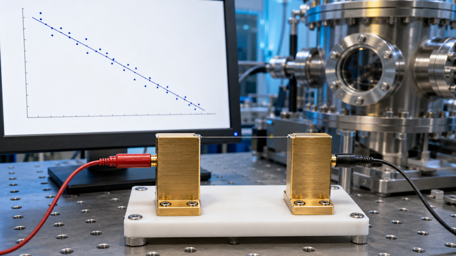
The logarithm that straightens the curve
The series solution that governs a TET transient is a sum of decaying exponentials with rates m²π²α/L² for odd m2. The m = 3 mode decays nine times faster than the fundamental, m = 5 twenty-five times faster; beyond a modest Fourier number the fundamental is effectively alone. In that regime the approach of the voltage to its steady-state value V1 is a single exponential in time, and the logarithm of the difference is exactly linear:
ln|V(t) − V1| = −π²αeff t / L² + D
The transformation costs nothing physically — it is the same data — but it changes the statistical character of the problem completely. A nonlinear fitting task with an iterative optimizer, a required starting guess and a convergence check becomes ordinary least-squares regression: closed-form, single-pass, with a century of well-understood statistics attached. The strong linearity of the transformed signal over the practical operating window has been demonstrated directly in the method literature3.
When is the single-mode regime actually reached? The mode ratios give a precise answer. Relative to the fundamental’s remaining transient, the m = 3 mode’s residual is (1/81) exp(−8π²Fo): it falls below roughly 0.25% by Fo = 0.02, below 0.024% by Fo = 0.05, and is utterly negligible — parts per million — by Fo = 0.10. Mathematically, then, the line straightens very early. The practical start of the regression window is set not by mode decay alone but by everything else that contaminates early data — current-source settling, amplifier bandwidth, endpoint estimation and the observed residual pattern — so the working rule is visual and self-enforcing rather than a universal Fourier-number threshold: plot the transform, find where straightness begins, and let the data choose the window’s start.
Slope to diffusivity
Reading the physics off the line is one step. The regression slope is −π²αeff/L², so
αeff = −slope · L² / π²
with L measured under a microscope. The subscript matters: what the slope delivers is the effective diffusivity of the experiment as performed — the effective response of the configured experiment, combining intrinsic transport with the parasitic channels and boundary conditions admitted by the measurement model — radiation chief among them for thin, high-emissivity samples. That is not a weakness of the linearization; it is a property of the physical measurement that every reduction route shares, and the TET family handles it head-on: the differential variants measure αeff across systematically varied lengths or coatings and extrapolate the loss channels away — the modern review maps these differential protocols from millimeter down to atomic-scale thickness4. The linear route can make each fitted slope’s statistical contribution to those extrapolations more explicit — each individual αeff can be accompanied by a regression-only standard error — provided the regression assumptions and the covariance between extrapolated points are handled correctly.
Regression uncertainty comes with the slope
Here is the practical center of the argument. Nonlinear least squares can also provide parameter covariance and standard errors under an explicit residual model5 — the advantage of the linearized route is not that uncertainty exists only there. The advantage is that the diffusivity comes from a closed-form slope whose residuals, leverage and regression-only standard error are easy to inspect and audit, with no optimizer settings, starting guesses or convergence tolerances to document; both analyses remain conditional on the chosen model, weighting, endpoint estimate and residual assumptions. In ordinary linear regression, the standard error of the slope is a standard textbook output, computed directly from the residual scatter and the spread of the time points. The uncertainty of αeff follows by the same constant factor L²/π² that converts the slope itself. One computation returns the fitted value and a transparent regression-only precision estimate. The slope’s standard error is the residual standard deviation divided by the square root of the summed squared deviations of the time points from their mean — a formula every statistics textbook prints and every spreadsheet implements, with a closed-form calculation throughout: the slope standard error follows from the residual variance and the leverage of the time points, avoiding iterative optimization and a Jacobian-based nonlinear covariance estimate, while remaining conditional on the residual model, independence assumptions and weighting used in the regression. And because a regression-derived precision estimate travels with the fitted value, results from different runs, samples or laboratories can be compared statistically when the measurand, residual model, uncertainty definition and coverage statement are comparable — precisely the discipline that cross-method comparisons of the same physical specimen demand6. For a commercial instrument intended to produce results that survive scrutiny — a datasheet challenge, a qualification audit, a customer’s own re-measurement — making the error bar a native output rather than a post-processing choice is precisely the design goal, and it is the property the patented analysis is built around1. It is also the property that matters most when results feed the verification protocols discussed in our claim-validation guide.
Fit-start stability within a validated window
Every analyst who has fit transients knows the quiet embarrassment: move the fitting window’s start a little and the answer moves too. For reduced-model nonlinear fits that sensitivity comes from the early-time region, where unmodelled fast modes can bias the fit; a full-series fit can represent those modes, yet may still be affected by instrument settling, endpoint estimation, weighting and other model discrepancies. The linearized route is structurally protected in expectation: within a validated linear window and under a correct endpoint estimate, a straight line has one slope wherever you start reading it. Truncating the first portion of the linear region changes which points enter the regression, but not the expected slope — the observed slope can still move with noise, endpoint error and residual curvature, which is exactly what the transform’s visible straightness lets you check. Insensitivity to the fitting start point is one of the explicit advantages of the linearized analysis1, and it converts a subjective analyst decision into a transparent statistical trade-off.
The operational payoff shows up in automation and in auditability. Within a validated linear region and with V1 correctly estimated, the expected slope remains comparatively stable as the fit start moves — the fit start does not affect only the error bar, since the selected points, noise realization, endpoint error and residual curvature all shift with it, but the shift is checkable. An automated implementation can choose the window by predeclared curvature and noise-floor criteria and apply the same prevalidated window-selection rule without requiring an operator to choose the boundary by eye, validating that window through residual inspection and repeated-window stability. And when a result is challenged months later, the audit trail is short: the raw transient, one transform, one regression, two numbers. Compare the equivalent audit of a nonlinear fit — optimizer settings, starting guesses, convergence tolerances, covariance approximations — and the linear route’s reproducibility advantage is not aesthetic; it is the difference between an argument and a recomputation.
Two honesty clauses keep this argument rigorous. First, ordinary least squares carries its own assumptions — independent, comparable-variance residuals on a correct model — and the logarithm works against them near steady state, where additive voltage noise becomes amplified and asymmetric in the transform; a disciplined implementation truncates the tail before the noise floor or applies weighting there — transformation and weighting being the two standard remedies for non-constant variance7. Second, the regression’s standard error is the regression-only uncertainty, one layer of a fuller budget:
| Uncertainty level | What it includes |
|---|---|
| Regression-only | Residual scatter and the time-point leverage of the fitted window |
| Reduction uncertainty | Steady-state (V1) estimation, window choice, weighting, model form |
| Experimental uncertainty | Sample length and geometry, voltage and time base calibration, boundary and radiation terms |
| Combined reported uncertainty | All relevant terms propagated together, per the GUM framework8 |
The linearized route’s genuine contribution is making the first layer closed-form, transparent and cheap — not making the other layers disappear.
What the patent actually claims
Stripped of legal formatting, the patented method covers the analysis chain this article has walked: acquire the voltage transient of a step-heated suspended sample; form the logarithm of the difference from the steady-state voltage; regress it linearly against time; obtain the effective thermal diffusivity from the slope through the sample geometry; and obtain a regression-derived uncertainty associated with the fitted thermal characteristic from the same operation1. The claims sit at the analysis layer, and — as with any patent — the published claims themselves, not this plain-language summary, define the legal scope; U.S. Patent No. 12,372,489 B2 includes claims directed to specified electrothermal measurement and processing workflows involving logarithmic transformation, linear regression and, in certain claims, uncertainty determination from that regression. The ThermalSure® TEPT X1 is the instrument built on it, and the standardized laboratory protocol that the analysis slots into is documented in the method’s published procedure9. The same linearization logic extends across the family: the photo-electro-thermal variant, which heats optically and senses electrically, produces transients amenable to the identical transform10, and richer configurations extract specific heat alongside conductivity from combined transient and steady-state information while keeping the analysis chain transparent11.
Where linearization needs care
Honest advocacy names its boundaries. (1) The regime must be reached: the line is only straight after the higher modes die; fitting before that point re-imports the early-time bias in logarithmic clothing. In practice the onset is visible — the transformed data curve into the line — and the regression window starts where straightness begins. (2) The noise floor bends the tail: as V(t) closes on V1, the difference shrinks toward the noise, and its logarithm turns systematic noise into asymmetric scatter; the window should close before the difference drowns. (3) V1 must be right: like the characteristic-point route, linearization consumes the steady-state value, and an error there curves the late line — visibly, which is itself a diagnostic. (4) Nonlinear physics stays nonlinear: radiation changes the effective response and must be corrected or extrapolated, while large temperature rises, strongly temperature-dependent properties or nonlinear radiative terms can introduce curvature that moves the experiment outside the validated linear model — a regime characterized within the method family12; the fix is experimental (smaller rise, differential configurations), not statistical — and the technique’s modern review maps exactly where those regimes begin across the materials record4. Even the temperature-readout assumption can be traded away when needed — the Johnson-noise variant of the family senses temperature without relying on resistance drift at all13. Within a validated fit window and a stated residual model, the transformed line is the welcome case where the simpler computation can also be the more auditable one — the method behind it is introduced in the TET complete guide, and the reduction landscape it improves on is mapped in the data-reduction companion.
Keep Exploring the ACS Thermal Metrology Knowledge Hub
This article is one chapter of the ACS thermal metrology knowledge hub. To keep going:
- Thermal conductivity & diffusivity testing: the pillar guide — methods, samples and a buyer’s framework in one place.
- From V–t curve to diffusivity — the three data-reduction routes compared.
- Zero-temperature-rise extrapolation — removing self-heating bias, validated on a Pt wire.
- Differential TET — correcting radiation, residual-gas transfer and coatings.
- ThermalSure® TEPT X1 — the instrument implementing this measurement family.
References
This article describes the linearized-regression analysis of TET transients in its idealized form; practical implementations add window-selection, radiation and coating considerations documented in the method literature and instrument documentation. Patent description is a plain-language summary, not legal advice; consult the published patent for authoritative claim language. The interactive simulator is a schematic teaching tool, not a substitute for measurement.