Bulk polymers are textbook insulators — a fifth of a watt per meter-kelvin, give or take — because their molecular chains lie tangled like cold spaghetti, and heat must rattle across weak van-der-Waals contacts at every turn12. Yet the individual chain is a stiff, light, covalent backbone — on paper, a superb one-dimensional conductor. Fiber drawing cashes that paper: stretch a polymer far enough and the chains comb into alignment, crystallites orient along the axis, and axial conductivity climbs by orders of magnitude in the best-documented systems — ultra-drawn polyethylene nanofibres have been measured at about 104 W m⁻¹K⁻¹, higher than many pure metals, and nanostructured polyethylene films at about 6234. This article walks the mechanism, the measurement problem a single micro-fiber poses — and the suspended electrothermal methods built to solve it56 — then closes with the caveats that keep spectacular fiber numbers honest on their way into datasheets.
| Measured directly | Thermal diffusivity α along the fiber axis (suspended electrothermal transient) |
|---|---|
| Derived | k = αρcp — not an independent measurement |
| Required inputs | Suspended length, cross-section, density, specific heat; coating properties if applied |
| Direction | Axial; transverse requires a separate measurement |
| Main corrections | Zero-power extrapolation, radiation, contacts, coating contribution |
| Reported uncertainty | State whether regression-only or combined |
Why tangled chains insulate and combed chains conduct
Follow one joule through amorphous polyethylene: it sprints along a covalent backbone for a few nanometers, hits a chain end or a fold, and must hop across a van-der-Waals gap an order of magnitude softer than the bond it left — then again, and again, thousands of times per millimeter. The macroscopic conductivity is the harmonic mercy of those hops, which is why nearly every bulk polymer lands in the same 0.1–0.5 W m⁻¹K⁻¹ corridor regardless of chemistry12. The chain itself was never the problem: simulations and single-chain estimates point to intrinsic backbone conduction far above the bulk, parked behind the interchain bottleneck — and high-modulus fiber studies show how much of that potential real processing can release27. Conduction physics thus hands polymer engineering an unusual lever — not chemistry, but order: reduce the hops per unit length, and the material remembers what its bonds can do.
What drawing actually does
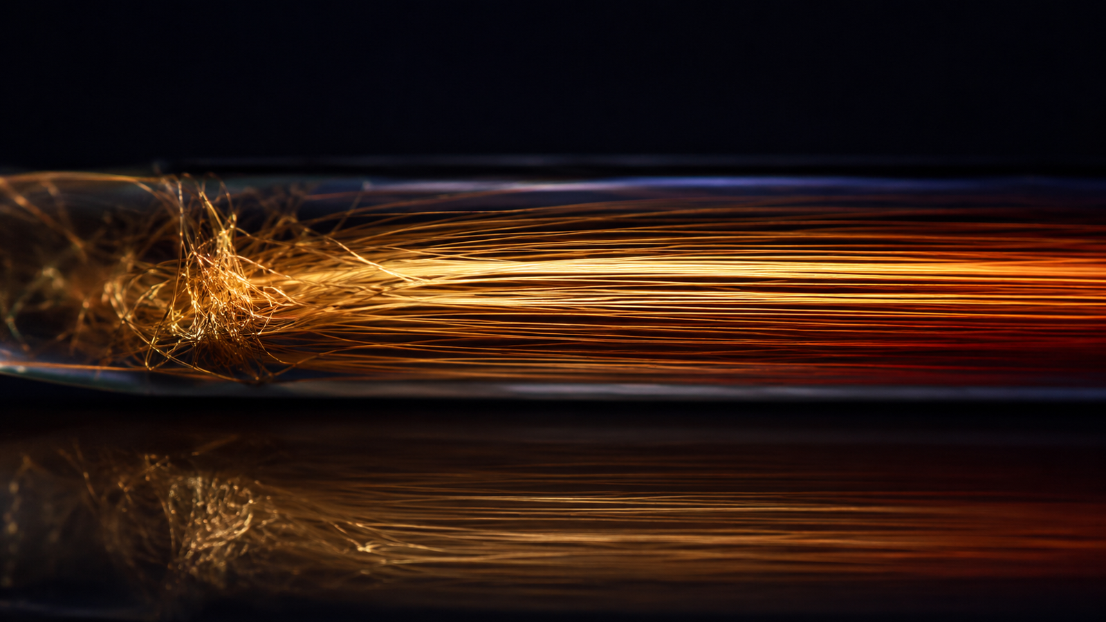
Mechanical drawing is that lever. Pulling a fiber to high draw ratio does three cooperative things: it uncoils and aligns amorphous chains along the axis, so a phonon’s covalent sprint lengthens before its next hop; it orients and extends crystallites, whose ordered interiors conduct far better than the amorphous sea; and it couples crystalline bridges through the structure, building near-continuous stiff pathways down the fiber28. Measured consequences track the structure: over the effective processing window axial conductivity rises steeply with draw ratio, with ultra-drawn polyethylene the celebrated extreme, reaching values comparable to structural metals along the axis37. The rise is not guaranteed to continue indefinitely — defects, voids and processing limits eventually cap it — and gains are strongly directional, with transverse conduction remaining far lower and set by the interchain contacts drawing never removes4. The gains are real, directional, and structure-fragile — three adjectives that preview both the measurement problem and the caveats below.
Interactive: alignment versus axial conductivity
The simulator animates the mechanism at cartoon scale: a field of chain segments whose orientations tighten toward the axis as you raise the alignment slider, while the readout curve translates alignment into relative axial conductivity through a simple series picture — the fewer interchain hops per unit length, the higher the axial channel climbs, with the radial channel pinned near bulk. Drag from tangled to combed and watch both the picture and the curve tell the same story.
The mapping is a schematic monotonic model built for intuition — real draw-ratio curves depend on polymer, crystallinity, molecular weight and processing route; the monotone rise and the axial/radial split are the transferable truths2.
Measuring one micro-fiber honestly
A drawn fiber tens of micrometers thick defeats every conventional platform — no disc to flash, no slab to press — and hands the job to the suspended electrothermal family, where the fiber itself becomes heater and thermometer. Bridge the sample between two electrodes, pass a current step, and the resistance transient times the axial diffusion; steady components deliver conductivity once geometry and losses are accounted56. For the non-conductive polymers that dominate this field, a thin metallic coating carries the current while a differential treatment accounts for it — not a simple subtraction, since the coating contributes both conductance and heat capacity and its own interface to the fiber69. The error budget has polymer-specific line items: radiation from high-emissivity surfaces (vacuum and radiation accounting are non-negotiable), contact quality at the mounts, and cross-section uncertainty on non-circular fibers — each with published countermeasures, from zero-power extrapolation to length-series differentials — noting that zero-power extrapolation addresses the self-heating bias specifically and does not absorb cross-section, contact or radiation errors, which need their own treatment610. Optothermal and microdevice routes triangulate the family on the smallest specimens11. The measurement is mature; what it demands is the same thing the material rewards — discipline about direction and structure.
The honest caveats: anisotropy, temperature, spread
Three caveats keep fiber numbers honest. Direction: the gains are axial; transverse conductivity remains far lower — typically in the ordinary polymer range for drawn fibers, though it is a measured quantity rather than a constant — so any application that heats across fibers — mats, weaves, composites loaded transversely — inherits the polymer-ordinary number, and datasheets must say which axis they mean2. Temperature and stability: alignment is a processed state, not a thermodynamic one; approach the polymer’s relaxation temperatures and the combed structure — and its conductivity — can retreat, so service-temperature data belong on the sheet. Spread: draw ratio, crystallinity and molecular weight scatter between lots, and the literature’s own spread across nominally similar fibers is the strongest argument for measuring your batch rather than citing a champion’s212. None of this diminishes the achievement — insulator chemistry conducting like metal along one axis is a genuine materials victory — it just relocates the datasheet from the press release to the measurement lab.
Frequently asked questions
How high can drawn polymer fibers actually go?
Ultra-drawn polyethylene nanofibres have been reported at roughly 104 W m⁻¹K⁻¹ and nanostructured polyethylene films at about 62 — two to three orders above the ~0.1–0.35 of bulk polyethylene34. Treat any specific figure as belonging to its draw ratio, structure, diameter and measurement method rather than to the polymer in general7.
Does the enhancement survive in composites?
Partially. Fiber-axis conduction survives along continuous, aligned reinforcement; junctions, matrix interfaces and transverse loading reintroduce the hops the drawing removed — the same interface arithmetic that governs nanotube networks13.
Which method measures a single polymer fiber?
Suspended electrothermal transients are a native route — delivering diffusivity, with conductivity following only once ρcp is supplied — with metallic-coating and differential protocols for non-conductive fibers; microdevice platforms take the smallest specimens59. The technique article covers the workflow end to end.
Why do radial and axial values differ so much?
Because drawing builds highways in one direction only: along the axis phonons ride extended covalent paths; radially they still hop van-der-Waals gaps at bulk frequency. The fiber is a deliberately anisotropic object and must be reported as one2.
Is chain alignment the only route to conductive polymers?
No — conductive fillers, crystallinity engineering and blending all contribute — but alignment is the route that upgrades the polymer itself rather than diluting it, which is why fiber drawing anchors the field’s headline results2.
Keep Exploring the ACS Thermal Metrology Knowledge Hub
This article is one chapter of the ACS thermal metrology knowledge hub. To keep going:
- Thermal conductivity & diffusivity testing: the pillar guide — methods, samples and a buyer’s framework in one place.
- The transient electro-thermal technique: a complete guide — the suspended-sample family at the heart of this hub.
- Testing non-conductive samples: the metal-coating protocol — making insulators measurable, then subtracting the film.
- Carbon nanotube thermal transport — ballistic heat and how it was measured.
- Thermal conductivity of graphene fibers — measurement and meaning for wet-spun filaments.
- Thin-film thermal conductivity: in-plane vs cross-plane — why one number is never enough.
- Thermal conductivity of biological fibers — hair, silk, cellulose and the moisture problem.
- ACS thermal testing services — the team that turns these distinctions into data on your specimen.
References
This article discusses polymer fiber thermal conductivity for educational purposes. Enhancement magnitudes are values reported in the cited literature for specific drawn fibers and films; they are directional (axial), structure- and processing-dependent, and transverse values are far lower but must themselves be measured rather than assumed. The alignment simulator is a schematic teaching model. Consult product datasheets and SDS, and contact our thermal testing team for fiber-specific data.