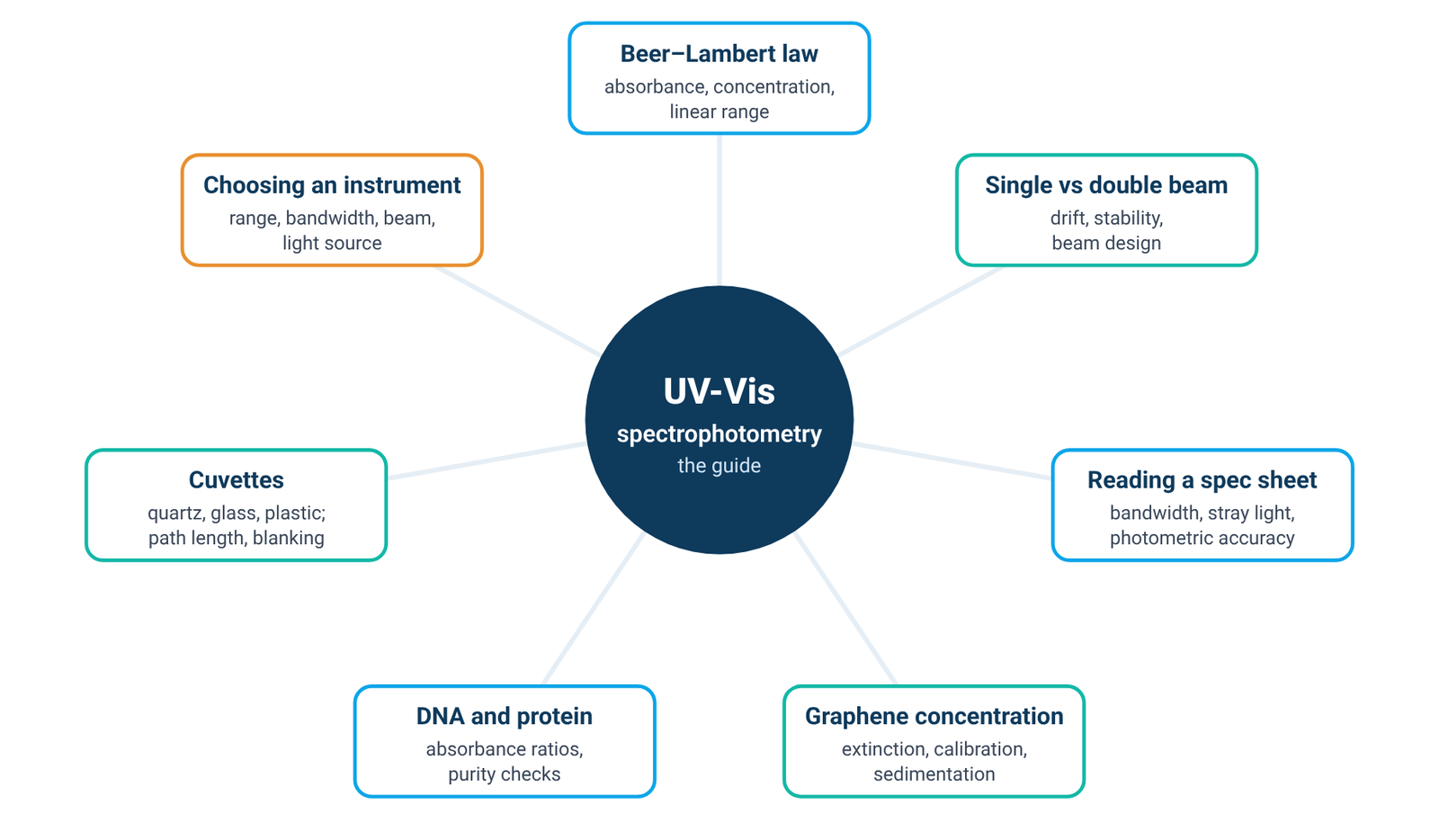
An absorbance reading measures light that is missing. The instrument compares how much light gets through your sample with how much gets through a blank, and reports the difference on a logarithmic scale. Whether that number means what you think it means depends on the light source, the monochromator, the optical layout, stray light and the sample itself. This guide walks through each of them in turn and points to the detailed guides in our UV-Vis hub.
Quick answer: UV-Vis spectrophotometry measures how much ultraviolet or visible light a sample removes from a beam, by comparing the light that reaches the detector through the sample with the light that reaches it through a blank [1][2]. The ratio is the transmittance, T = I/I₀, and absorbance is A = −log T [2]. Every dispersive instrument is built from four blocks: a light source, a monochromator that selects a narrow band of wavelengths, the sample, and a detector [1][2]. How accurate the absorbance is depends on the source and its stability, the spectral bandwidth, stray light, and the sample and cuvette; Harvey gives 0.1–1 as a practical range for about ±1–2 % relative uncertainty in concentration [5].
1. What UV-Vis Spectrophotometry Measures
A spectrophotometer is an instrument for measuring the transmittance or absorbance of a sample as a function of wavelength [1]. In UV-Vis work that means light from the ultraviolet through the visible region; the Agilent primer describes the typical span as 190 to 900 nm [2], although the range of any particular instrument is set by its source, optics and detector. At each wavelength, the instrument measures the intensity of light reaching the detector without the sample, the blank, and compares it with the intensity after the light has passed through the sample [1]. Transmittance is the ratio T = I/I₀, often quoted as %T, and absorbance is A = −log T [2]. Because the scale is logarithmic, an absorbance of 1 means that one tenth of the light gets through, and an absorbance of 2 means that one hundredth does.
Strictly, the reading is light that did not arrive at the detector, not light proven to have been absorbed. When radiation meets matter, several things can happen: reflection, scattering, absorption, absorption followed by re-emission as fluorescence or phosphorescence, and photochemical reactions [2]. Anything that diverts light away from the detector raises the apparent absorbance. For a clear solution measured against a blank of the same solvent in the same type of cell, most of these losses are shared by blank and sample and cancel [1][2]. For turbid samples, cells or nanomaterial dispersions they do not: scattering produces an apparent background absorbance even where nothing absorbs [1], and what the instrument records is better described as extinction, the sum of absorbance and scattering [6].
For quantitative work, absorbance is linked to concentration by Beer's law, A = εbc, where ε is the molar absorptivity, b the path length and c the concentration [2][4]. Our Beer–Lambert law formula guide covers units, worked examples and the linear range in detail. Two practical points belong here. First, predetermined absorptivity values are usually not used for quantitative analysis; instead, a calibration or working curve is prepared from standards measured on your own instrument [2]. Second, the relationship is most useful inside a limited window: to obtain a relative uncertainty in concentration of about ±1–2 %, Harvey recommends keeping the absorbance within the range 0.1–1 [5].
Beer's law also has known limits. Harvey groups them as fundamental, chemical and instrumental, and lists polychromatic radiation and stray radiation among the instrumental causes of deviation [4]. Both of those come from the design of the instrument, which is why the next four sections look at how a spectrophotometer is built before returning to the sample in section 6.
2. How a UV-Vis Spectrophotometer Works: The Four Blocks
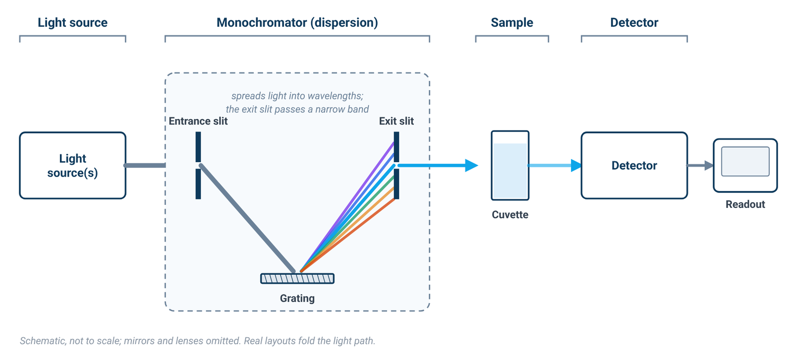
Every dispersive UV-Vis spectrophotometer contains the same four functional blocks: a light source; a dispersion device that separates the broadband radiation into wavelengths; a sample area; and one or more detectors [1][2]. The way these blocks are arranged, and the quality of each one, explains most of what appears on a specification sheet.
The light source
The source has to emit useful intensity at every wavelength the instrument is asked to measure. No single conventional lamp does this well across both the ultraviolet and the visible, which is why most UV-Vis instruments carry two lamps [1]. Section 3 looks at the lamp types and what each one covers.
The monochromator
The monochromator selects the wavelength. It consists of an entrance slit, a dispersion device and an exit slit [1][2]. Light enters through the entrance slit, the dispersion device spreads it out by wavelength, and the exit slit passes a narrow portion of that spread on to the sample. Holographic diffraction gratings are now the usual dispersion device in place of prisms, and they give a linear angular dispersion with wavelength [1][2]. A grating also produces overlapping orders of diffraction, so filters are used to remove unwanted orders [2].
Ideally the monochromator would deliver a single wavelength. In practice, the output is always a band of wavelengths [1][2]. The width of that band at half its height is the instrumental bandwidth, usually called the spectral bandwidth [1], and it is set primarily by the widths of the entrance and exit slits [1]. That one fact runs through much of this guide: the instrument never measures at a single wavelength, so the shape of the sample's absorption band and the width of the instrument's band interact (section 5).
The sample area
The sample compartment holds the cuvette in the beam. Standard cuvettes have a 10 mm path length [2]. The inside of the compartment is usually matt black, which helps to absorb stray light [2]. In a double-beam instrument the compartment also holds a second cell for the reference (section 4).
The detector
The detector converts the transmitted light into an electrical signal. Photomultiplier tubes and silicon photodiodes are both used; photodiodes have a wider dynamic range and are more robust than photomultipliers [1][2]. The limits of detection for silicon-based detectors are approximately 170 to 1100 nm [1][2]. The detector and the source together decide how small a change in light can be measured reliably. This matters most at high absorbance, because very little light then reaches the detector and the signal-to-noise ratio falls [2].
Scanning and diode-array layouts
In the layout described above, the instrument measures one band at a time and steps or scans through wavelengths. Other designs exist: a diode-array spectrometer measures many wavelengths at once and can record a full spectrum in as little as 0.1 s [5]. The questions in the rest of this guide, about sources, beam design, bandwidth and stray light, are framed around the monochromator-based design, because that is where the specification lines discussed in section 5 come from.
3. Light Sources: Tungsten, Deuterium and Xenon
A UV-Vis source has to provide a continuum, with enough intensity at every wavelength the monochromator might select. In most instruments two conventional lamps share the work. A deuterium arc lamp yields a good intensity continuum in the UV region and provides useful intensity in the visible region [1][2]. A tungsten-halogen lamp yields good intensity over part of the UV spectrum and over the entire visible range, and continues into the near-infrared [1][2]. Most spectrophotometers used to measure the UV-visible range therefore contain both types of lamp [1].
Textbook figures for the usable ranges differ a little between sources. Harvey lists a hydrogen or deuterium lamp continuum from 160–380 nm and a tungsten lamp continuum from 320–2400 nm [3]; the Agilent primer gives 185 to 400 nm for deuterium and 350 to 3000 nm for tungsten-halogen [2]. The exact numbers depend on the lamp and the reference, but the picture is the same in each: deuterium covers the ultraviolet, tungsten covers the visible and near-infrared, and the two overlap in the near UV.
The practical consequence follows directly from those ranges. A tungsten source on its own does not reach far into the ultraviolet, so measurements below roughly the lower end of its range need a deuterium or other UV source [2][3]. When you read an instrument listing, the light-source line should therefore be read together with the specified wavelength range; a tungsten-only listing should not be assumed to cover the deeper UV.
A xenon lamp offers a different route to the same coverage: a single lamp that yields a good continuum over the entire UV and visible regions [1][3]. In an instrument listing, "xenon lamp" therefore tells you that one source covers both regions, where a two-lamp design uses deuterium for the UV and tungsten for the visible. Which arrangement suits a given laboratory is one of the four choices compared in our buying guide (section 8). For the measurement itself, what matters is that the source covers your wavelengths with enough light at each.
Whatever the lamp, its output is not perfectly constant. Lamp intensity changes over medium and long timescales, which Owen calls drift [1]. In a single-beam instrument, any change in light intensity between the blank reading and the sample reading appears as an error in the measured absorbance [2]. That is the problem the double-beam layout was developed to address.
4. Single-Beam vs Double-Beam Instruments
A conventional single-beam instrument has one light path. Absorbance is determined by measuring the intensity of light reaching the detector without the sample, the blank, and comparing it with the intensity of light reaching the detector after passing through the sample [1]. Because the two readings are taken at different times, the method assumes that nothing in the instrument changed in between. If there is any variation of light intensity, or of system optical performance, between the baseline and the sample reading, the measurement may be less accurate [2]. Harvey puts it directly: the accuracy of a single-beam spectrophotometer is limited by the stability of its source and detector over time [5]. The remedy is procedural. With a single-beam system, a baseline or blank measurement should be run frequently and regularly during a measurement session [2].
The single-beam layout is not simply the cheaper option. Single-beam instruments are low in cost, and the simple optical system offers high throughput and hence high sensitivity [1]. Owen also notes that the reference spectrophotometers used by national standards institutions such as NIST in the United States and NPL in the United Kingdom are single beam [1].
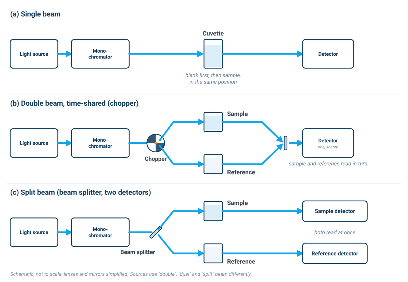
In a double-beam instrument, the light leaving the monochromator is split into two beams, a reference beam and a sample beam [2]. In Harvey's description, a chopper controls the radiation's path, alternating it between the sample, the blank and a shutter [5]. Because the reference is measured alongside the sample, the sample measurement can be corrected for instrument fluctuations in real time [2]. Owen describes the purpose plainly: the dual-beam design was developed to compensate for changes in lamp intensity between measurements on the blank and sample cuvettes, correcting for medium- and long-term changes in lamp intensity [1].
The cost is complexity. The dual-beam layout has more optical components, which reduces throughput and sensitivity [1]. Double-beam instruments are more versatile than single-beam instruments, but they are also more expensive and not particularly portable [5].
It is just as important to know what the reference beam does not do. It compensates for changes that the two beams share, in the lamp and the electronics [1][2]. It does not compensate for a change that occurs only in the sample cell, such as particles settling or the sample itself changing during the measurement. Nor does the beam layout set stray light: stray light is reduced by the monochromator and optical design, for example by a double monochromator [2], not by adding a second beam. Our single beam vs double beam spectrophotometer guide goes through drift, stability specifications and the situations where the choice matters.
5. Reading the Specification Sheet: Bandwidth, Stray Light and Photometric Range
Three groups of specification lines say most about whether an instrument will measure your samples accurately: spectral bandwidth, stray light, and the photometric lines (accuracy and range). Each one is well defined in the literature, and each one is easy to over-read. Our guide to reading a spectrophotometer spec sheet goes line by line; this section covers the principles.
Spectral bandwidth
Because the monochromator passes a band rather than a line, the spectral bandwidth (SBW) is defined as the width of that band at half its height [1]. SBW is primarily a function of the entrance and exit slit widths [1], and for double-beam scanning instruments Harvey notes that effective bandwidths of 0.2–3.0 nm are common [5].
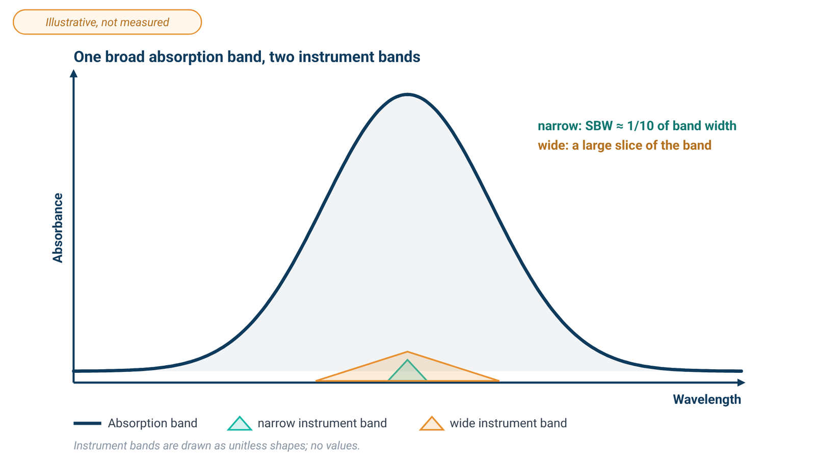
What matters is not the bandwidth alone but its ratio to the natural bandwidth (NBW) of the absorption band you are measuring. Owen states that an SBW/NBW ratio of 0.1 or less will yield an absorbance measurement with an accuracy of 99.5 % or better [1], and the Agilent primer gives the same working rule: set the SBW to approximately one tenth of the natural bandwidth of the analyte [2]. Most solid or liquid samples have naturally broad peaks, of the order of 20 nm or more [2]. A larger SBW allows more light through the sample, but it will not resolve narrow or closely spaced peaks [2].
The narrowest bandwidth on offer is therefore not automatically the right one. For the broad bands typical of solutions, the one-tenth rule is met without going to the narrowest setting an instrument family provides; a narrower bandwidth matters when the sample has narrow or closely spaced peaks [2]. Match the bandwidth to your spectra rather than to the smallest number on a specification sheet.
Stray light
Stray light, or stray radiant energy, is defined as the percentage of radiation reaching the detector whose wavelengths are outside the selected spectral band [2]. It matters most where the sample absorbs strongly. The stray light still reaches the detector, so the detector receives more light than the selected band alone would deliver, and the absorbance reads low [2]. Owen describes the effect as a negative bias in the measured absorbance [1], and it is one of the instrumental causes of deviation from Beer's law [2][4]. Stray light also determines the maximum absorbance an instrument can measure [2].
Stray light is controlled by the optics. A matt-black sample compartment helps to absorb it [2], and a double monochromator reduces it [2]. It is not a property of the beam layout, which is why section 4 did not list it among the things a reference beam corrects.
Photometric range is not the linear range
A specification sheet also gives a photometric range: the span of absorbance values the instrument will report. Owen's definition is blunt: the instrument range is simply the numerical range an instrument can display [1]. That is not the range over which absorbance is proportional to concentration, and it is not the range in which readings are most accurate. At high absorbance very little light reaches the detector, which decreases the signal-to-noise ratio [2], and stray light biases readings downward [1][2]. The working range for quantitative work is therefore much narrower than the displayed range. Harvey's 0.1–1 guideline from section 1 is a sound default [5], and the linear range of your own method is something to establish with standards [2].
On photometric accuracy, the Agilent primer makes a point that is easy to miss. In quantitative analysis, the calibration process should eliminate instrumental bias, which makes absolute photometric accuracy relatively unimportant; photometric reproducibility, on the other hand, is essential, and the instrumental linear range is critical [2]. A calibration curve made on the same instrument, under the same conditions, is what turns a reading into a concentration.
6. Getting Accurate Absorbance: Cuvettes, Blanks and the Sample
Once the instrument is chosen, the reading still depends on what you put in the beam and how you reference it.
Choose the cell for the wavelength
Standard cuvettes have a 10 mm path length and are made from quartz [2], which is the material for ultraviolet work. Cheaper plastic cuvettes generally do not transmit UV light [2], and glass absorbs strongly below 320 nm, so it is not suitable for measurements in that region [1]. Our quartz vs glass cuvette guide covers cell materials, path lengths and handling.
Make the blank match the sample
The blank defines the reference intensity, so it should contain everything the sample contains except the analyte. If the sample is simply an analyte dissolved in a pure solvent, use that pure solvent as the blank [1][2]. In a double-beam instrument the reference cell carries the blank; Owen describes a balance measurement in which both cuvettes are first filled with pure solvent before the sample cuvette is filled with sample [1].
Check the solvent
The solvent sets a lower wavelength limit of its own. Water allows measurement throughout the UV wavelengths, while the use of organic solvents limits the usable UV range [2]. A blank that absorbs strongly near its cut-off leaves little light for the measurement, so treat readings close to a solvent's limit with caution.
Keep the absorbance in range
If a sample reads high, do not trust the displayed number simply because the instrument can show it. At high absorbance very little light reaches the detector [2]. Diluting the sample is one way to bring the measurement into the linear range; alternatively, use a shorter path-length cuvette [2]. Harvey gives 0.1–1 as a practical range for about ±1–2 % relative uncertainty in concentration [5]. Very low readings fall outside the same window [5], and a longer path or a more concentrated sample may help there.
Watch for scattering
Turbid samples need care. Scattering causes an apparent absorbance because light is scattered at an angle instead of passing through the solution to the detector [1]. Small particles scatter in inverse proportion to the fourth power of the wavelength and large ones to the square of the wavelength, so the error due to scattering increases at lower wavelengths [1]. Filtering samples before measurement eliminates scattering but may not always be practicable [1]. A baseline that rises toward the ultraviolet can be a sign of scattering, and for particulate dispersions it is a reason to distinguish extinction from true absorbance.
7. Where UV-Vis Is Used
The same measurement serves very different fields. Three examples from our UV-Vis hub show how the principles above play out in practice.
Nanomaterial dispersions
For graphene, graphene oxide and nanoparticle dispersions, the instrument records extinction rather than pure absorbance: extinction is the sum of absorbance and scattering, and almost all experiments on such dispersions actually measure extinction [6]. The coefficient that links extinction to concentration can depend on nanosheet size as well as on wavelength [6], so a concentration needs a calibration made on your own dispersion. Our guide to graphene concentration by UV-Vis covers wavelength choice, calibration and sedimentation.
Nucleic acids and proteins
In life-science laboratories, UV absorbance is used to quantify nucleic acids and proteins and to screen their purity. The ratio of absorbance at 260 nm and 280 nm is used to assess the purity of DNA and RNA, and a ratio that is appreciably low may indicate protein, phenol or other contaminants that absorb strongly at or near 280 nm [7]. These measurements sit in the ultraviolet, so they need a UV source and quartz cells (sections 3 and 6). The A260/A280 ratio guide explains the ratios, what they can and cannot show, and how to measure them.
Thin films and surfaces
UV-Vis is used on solids as well as liquids: to characterize the absorbance or transmittance through a liquid or solid, and the reflectance properties of a surface [2]. For coatings and thin films, reflectance and transmittance spectra are also one input to thickness measurement by optical interference, which our article on how to measure thin film thickness covers alongside profilometry and ellipsometry.
8. Choosing an Instrument
Choosing a spectrophotometer comes down to matching four things to your samples: wavelength range, spectral bandwidth, beam design and light source. The ALab range currently includes ten spectrophotometer models. The ALab SP-1000/1100 series includes four single-beam models with a dot matrix LCD: the SP-UV1000 and SP-UV1100 use tungsten and deuterium lamps, while the SP-V1000 and SP-V1100 use a tungsten lamp only. The other six are individual models: SP-UV2101 (single-beam, touch screen); SP-UV2102, a single-beam touch-screen instrument with tungsten and deuterium lamps; SP-UV3101 and SP-UV3102, double-beam touch-screen instruments with tungsten and deuterium lamps; and SP-XUV5101 and SP-XUV5102, double-beam touch-screen instruments with a xenon lamp. Across the range, six models are single-beam, four are double-beam, and two use a xenon lamp. Spectral bandwidth, stray light and the photometric lines differ from model to model and should be read for each model against the rules in section 5, together with the wavelength range you actually need. Our guide on how to choose a UV-Vis spectrophotometer compares wavelength range, bandwidth, beam design and light source model by model.
9. Frequently Asked Questions
What is the difference between UV-Vis spectroscopy and UV-Vis spectrophotometry?
The terms are often used interchangeably. Spectrophotometry refers to the quantitative measurement itself: a spectrophotometer measures the transmittance or absorbance of a sample as a function of wavelength [1].
Why do I need a blank?
Absorbance is calculated by comparing the light reaching the detector through the sample with the light reaching it without the sample [1]. If the sample is simply an analyte dissolved in a pure solvent, use that pure solvent as the blank [1][2], so that the reading reflects the analyte rather than the solvent and cell.
Should I use a single-beam or a double-beam instrument?
A single-beam instrument has a simpler optical path and higher throughput, but its accuracy is limited by source and detector stability, so it needs frequent re-blanking [1][2][5]. A double-beam instrument corrects for lamp drift in real time but not for changes in the sample itself, and it does not reduce stray light [1][2]. See section 4.
Which cuvette should I use?
Quartz for ultraviolet measurements; plastic cuvettes generally do not transmit UV light [2], and glass absorbs strongly below 320 nm [1]. A 10 mm path length is standard [2]. See section 6.
What absorbance range is reliable?
As a guideline, keep the absorbance between 0.1 and 1 for a relative uncertainty in concentration of about ±1–2 % [5]. The photometric range on a specification sheet is the numerical range the instrument can display [1], not the linear range.
Do I need a very narrow spectral bandwidth?
Usually not for solutions. The working rule is an SBW of about one tenth of the natural bandwidth, and most liquid samples have bands of about 20 nm or more [1][2]. A narrow bandwidth matters for narrow or closely spaced peaks [2].
10. Keep Exploring the UV-Vis Hub
- Beer–Lambert law formula: absorbance, concentration and the linear range: units, worked examples and where linearity ends.
- Single-beam vs double-beam UV-Vis spectrophotometers: drift, stability and when the beam design matters.
- Spectral bandwidth, stray light and photometric accuracy: reading a spectrophotometer spec sheet.
- Graphene concentration by UV-Vis: extinction, calibration and sedimentation for dispersions.
- DNA and protein quantification by UV absorbance: the A260/A280 ratio, A260/A230 and purity checks.
- Quartz vs glass vs plastic cuvettes: cell material, path length and blanking.
- How to choose a UV-Vis spectrophotometer: wavelength range, bandwidth, beam design and light source.