Every measurement family eventually meets a sample that seems designed to defeat it. For suspended-sample electrothermal methods that sample is a single atomic layer: it can span micrometer-scale openings but not the millimeter-scale gauges of conventional suspended-wire work, it may not conduct electricity, and its thermal conductance is so small that almost anything touching it conducts more. The differential architecture answers all three objections with a support membrane and a composite-conductance decomposition — and in doing so pushes an approach that began with millimeter wires down to the atomic-thickness limit, where it complements the optical methods that otherwise own this territory.
- 1Three ways an atomic layer defeats a measurement
- 2The support-membrane architecture
- 3Support control and composite-conductance recovery
- 4Interactive: the differential error budget
- 5What it has measured
- 6Why supported-state transport is often the engineering number
- 7Where it sits among 2D thermal methods
- 8Frequently asked questions
- 9Keep exploring the knowledge hub
- 10References
Three ways an atomic layer defeats a measurement
Suspended-sample methods ask their samples to do three things: span a gap, participate electrically, and dominate the measured signal. On the first, precision matters: atomically thin sheets can be suspended over micrometer-scale holes and trenches — that is how the landmark free-standing measurements were made — but they cannot routinely bridge the millimeter-scale gauge lengths of conventional suspended-wire measurement with useful yield, robustness and signal share. On the second, conductive 2D materials such as graphene can carry the heating current and the resistance signal themselves — an added heater/sensor coating is required only for insulating or inadequately conductive 2D systems, and it then brings the whole correction apparatus of the coating protocol with it. And the third failure is arithmetic: an atomically thin conductor moves so little heat in absolute terms that clamps, residues and supports all threaten to out-conduct the thing being measured1. Any workable architecture must supply mechanical support, an electrical path and a signal-accounting scheme that keeps the sheet visible inside the total.
The support-membrane architecture
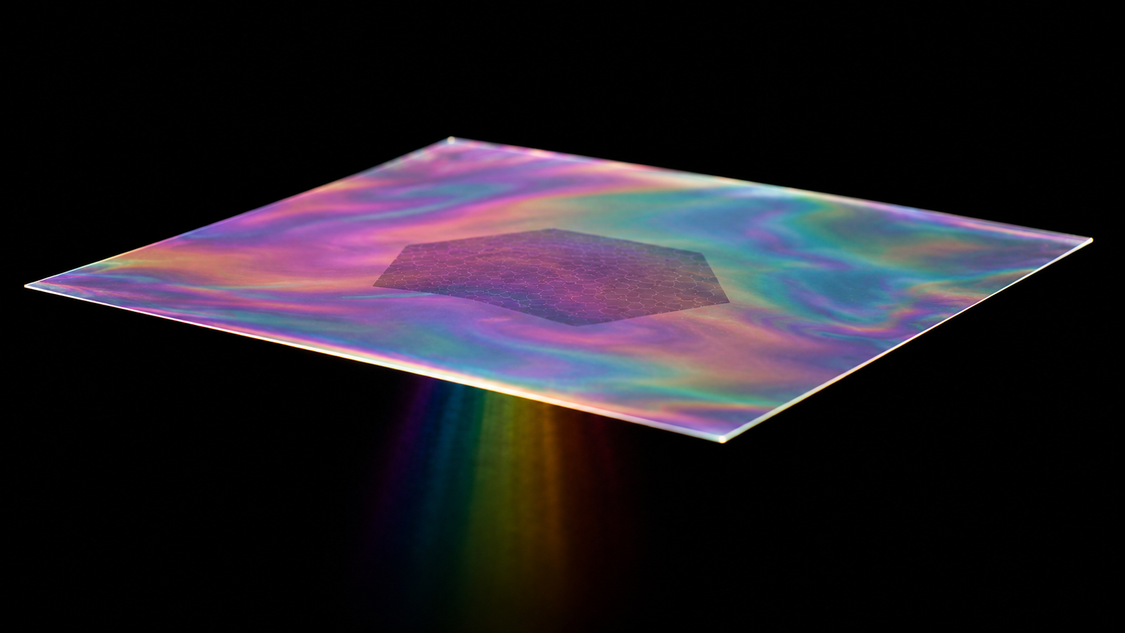
The differential architecture supplies the mechanical bridge and the signal-accounting framework at once; the electrical path comes either from a conductive 2D layer itself or from a separately characterized transducer for an insulating system. An ultrathin polymer membrane — poly(methyl methacrylate) at hundreds-of-nanometers thickness is the established choice — is suspended across the measurement gap as a carrying bridge. The 2D sample rides on the membrane. For a conductive sheet such as graphene, the sheet itself supplies the electrical path for Joule heating and resistance sensing; for insulating 2D systems, a nanometer metallic coating applied per the coating protocol takes that role — and adds its own correction problem to the budget2. The composite — support, sample, coating — is then a perfectly ordinary suspended specimen for the standard transient measurement3, reduced through the standard routes4.
The support’s thinness is not vanity; it is signal accounting. Every nanometer of membrane adds parallel conductance that the subtraction must later remove, and the removal’s health depends on the sheet’s share of the total staying appreciable. Hundreds of nanometers of low-conductivity polymer is the working compromise: robust enough to bridge and carry, thermally modest enough that an atomically thin high-conductivity sheet still announces itself in the composite’s transport1.
Transfer quality is the architecture’s silent variable. The sheet arrives on the membrane through a transfer step, and everything about that step — residue left by handling layers, wrinkles and folds that change the conducting cross-section, trapped contamination at the sheet–membrane interface — lands inside the “sample” term of the eventual subtraction. The discipline mirrors good 2D device practice: minimize and standardize handling chemistry, inspect the transferred region before committing it to measurement, and treat visible wrinkling not as cosmetic but as a geometry error in the making. A differential method can subtract the support it measured; it cannot subtract damage it never itemized.
Support control and composite-conductance recovery
The reduction is a composite-conductance model, and stating it in the additive quantity keeps it honest: axial conductances add, Kcomposite = Ksupport + K2D, while diffusivities do not subtract directly — converting the measured effective transport into channel conductances requires the support’s properties, both cross-sections and the composite heat capacity. In practice: determine the supported composite’s transport; quantify the support’s contribution from a separately validated support property or a matched control — ideally the same membrane characterized before transfer, or an identically processed twin; then recover the 2D contribution through the explicit composite model, whose details depend on whether the layer is uniform, electrically continuous and well coupled to the support1. The published graphene-on-PMMA campaigns follow exactly this modeled-composite route — support properties and layer-number distributions entering an explicit reduction, radiation handled by the length-differential analysis — rather than a literal two-number subtraction of paired measurements; the paired-control design this article describes is the idealized laboratory discipline toward which that modeling points.
Why sheet thermal conductance is more fundamental than W/mK for an atomic layer
For a sheet a few atoms thick, the conversion from measured conductance to a quoted conductivity divides by a thickness that is a convention — customarily the graphite interlayer spacing per layer — not a measured dimension. Two laboratories agreeing perfectly on the sheet’s axial or areal conductance can differ in W m⁻¹ K⁻¹ purely through bookkeeping. Reporting sheet thermal conductance first, with the thickness basis stated alongside any derived conductivity, is therefore the more fundamental — and more comparable — way to publish an atomic layer’s thermal transport.
Differential designs live and die by identicality, and every clause matters. Identical conditions means the same temperature, the same vacuum, the same mounting practice — anything that shifts the support’s own transport between the two measurements masquerades as sample signal. The same or twin support matters because membrane-to-membrane variation enters the subtraction at full strength. And because the answer is a difference of comparable quantities, the error-propagation arithmetic is unforgiving: uncertainties of both measurements combine, then divide by the sheet’s often-small share. This is the regime where per-transient regression-level precision4 and multi-current zero-rise discipline1 stop being refinements and become the difference between a number and noise. The uncertainty framework’s combination rules make the design constraint quantitative: independent variances add in the difference, then the sum divides by the sheet’s share, so in the low-share regime, halving per-measurement noise or roughly doubling the sheet’s share buys a comparable factor in the final budget5 — outside that limit the exact share-dependent expression governs — and those are the two levers the architecture and the protocol respectively control.
Interactive: the differential error budget
What it has measured
The architecture’s credentials are concrete: the modern review documents the differential approach extending electrothermal characterization down to atomic-scale thickness, with graphene on ultrathin PMMA bridges characterized across mono- to few-layer samples through the composite reduction1 — where the recovered values track sample quality and layer structure, not a simple “fewer layers, lower number” rule. Supported values sit well below the celebrated free-standing graphene figures — and should. The landmark measurement of monolayer graphene on silicon dioxide established the pattern: roughly 600 W m⁻¹ K⁻¹ near room temperature — far beneath suspended-flake values6 yet still above copper — with the suppression traced to phonons leaking across the graphene–support interface and interface scattering of flexural modes7. The pattern reproduces across preparations: CVD-grown monolayers measured in both suspended and supported states — transferred, fittingly, via PMMA handling layers — show the same substrate-induced suppression from a different growth route and measurement technique entirely8. The supported number is therefore not a lesser measurement of the same quantity but the honest value of a different, application-relevant configuration. Devices use supported sheets far more often than suspended ones; a method that measures the sheet as supported is measuring the configuration engineers actually deploy. The broader electrothermal family’s time resolution has also been leveraged for in-situ campaigns — tracking transport in graphene-family fibers continuously during laser photoreduction9 — the kind of dynamic measurement a slow method cannot attempt, and a capability adjacent to, though not specific to, the supported-2D architecture itself.
Why supported-state transport is often the engineering-relevant number
The distinction between free-standing and supported values is not academic bookkeeping; it decides which number belongs in a thermal design. Graphene’s commercial thermal formats — heat-spreader films, coatings, laminated stacks — deploy the material pressed against substrates, adhesives and encapsulants, and the application literature evaluates those films in exactly such supported, integrated configurations10. A datasheet built on suspended-flake values flatters every one of those products; a differential measurement of the sheet as supported prices in the substrate interaction the deployed material actually experiences. The two configurations answer different questions — and the supported one is usually the question the thermal designer is asking, a distinction the graphene thermal-management article develops on the application side and the claim-validation article turns into buying discipline.
Two further structure-sensitivity results sharpen the point. Micrometer-thick graphene-based films exhibit an intrinsic in-plane/through-plane anisotropy ratio that is itself a measured, structure-dependent quantity rather than a constant to be assumed11 — so “the conductivity of graphene” is underdetermined until orientation and stacking are specified. And carbon nanotube bundles have shown that processing state can move thermal transport by an order of magnitude within nominally the same material12. Against that backdrop, a method that measures the specific sheet, in its specific supported state, at its specific processing point, is often the most directly design-relevant measurement available for supported films, coatings and laminated devices — while suspended intrinsic values keep their own role in materials physics, free-membrane applications and model calibration.
Where it sits among 2D thermal methods
Two-dimensional thermal metrology is plural, and honest placement beats advocacy. Raman thermometry reads temperature optically from the sheet itself and pioneered suspended-graphene measurements6; its temperature scale rests on the Raman-shift calibration and laser-absorption estimates, which dominate its error budget. Time-domain thermoreflectance excels for supported films, multilayers and interfaces, with sensitivity governed by modulation frequency, transducer and the multilayer model13. The 3ω method brought lock-in rigor to thin films on substrates decades earlier and remains a reference point for cross-plane film metrology14. The differential electrothermal route’s distinctive offer is an electrically read, transient, regression-auditable measurement of a supported sheet — with the modern review noting that, where its geometry applies, its precision compares favorably against optical-calibration-limited alternatives1. The mature laboratory treats the three as complements sorted by sample format and question, a selection logic the pillar guide lays out in full.
| Aspect | Differential TET (this article) | Optothermal Raman | TDTR |
|---|---|---|---|
| Thermometer | Electrical resistance of the conductive 2D/support stack — or of a separately characterized transducer coating for insulating systems | Raman peak shift of the sheet itself6 | Optical reflectance of a metal transducer13 |
| Sample state addressed | Supported on the measuring membrane — the deployed configuration | Suspended or supported, per the thermal model and optical calibration8 | Supported films, multilayers, buried interfaces |
| Dominant error sources | Support reproducibility; difference-of-comparables amplification5 | Raman temperature calibration; absorbed-power estimate | Transducer & multilayer model parameters; spot metrology |
| Signal domain | Time-domain transient, regression-auditable4 | Steady-state optical, power-sweep based | Picosecond pump–probe, frequency/delay domain |
| Distinctive extra | Electrically read transient with regression-auditable fits; the broader electrothermal family adds in-situ dynamic capability9 | Simultaneous strain/doping spectroscopy from the same spectra | Film conductivity, interface conductance, or a correlated combination — per thickness, modulation frequency and sensitivity |
The decade in which all three matured — surveyed in the field’s second canonical review15 — settled the larger question by dissolving it: no single method owns 2D thermal metrology, and the credible datasheet is the one whose method was chosen to match the sample’s state and the question asked.
On the service side, contact our 2D material testing team to evaluate whether a sample suits a supported-composite or differential characterization workflow; the offering connects to the bulk materials service where the same family’s larger-format methods apply. The chain of ideas arriving here — transient model, reduction, regression uncertainty, parasite subtraction, coating protocol — runs through the whole TET series, and this article is where all of them are asked to perform at once.
Frequently asked questions
Keep Exploring the ACS Thermal Metrology Knowledge Hub
This article is one chapter of the ACS thermal metrology knowledge hub. To keep going:
- Thermal conductivity & diffusivity testing: the pillar guide — methods, samples and a buyer’s framework in one place.
- The metal-coating protocol — thermal testing for non-conductive samples.
- Graphene for thermal management — heat-spreader films, fibers and composites.
- Validating a heat-spreader claim — turning datasheet numbers into buying discipline.
- 2D material testing service — supported-composite characterization for atomic-thickness samples.
References
This article describes the differential support-membrane approach to 2D-material thermal characterization in general, idealized terms for education. Real campaigns involve transfer-quality control, support reproducibility validation and full differential uncertainty budgets; consult the published protocols and service documentation for specifics. The interactive tool above is a schematic teaching aid, not an instrument.