
Most compact cooled in-situ stages answer to one of two machines — the pair this article compares; closed-cycle cryocoolers and helium systems serve a different hardware class below the nitrogen floor. The first is a dewar of liquid nitrogen: a cryogen at −196 °C plumbed to the sample platform, brutal in reach, demanding in logistics. The second is a thermoelectric (Peltier) element: a solid-state slab that pumps heat when current flows, modest in reach, effortless in operation. Between them sits one of the most common purchasing decisions in the stage world — and one of the most commonly muddled, because the right answer depends less on which technology is “better” than on where your coldest required temperature actually lies. This article is the decision, laid out properly: how each method works, what each genuinely costs, and a decision tree you can walk in two minutes.
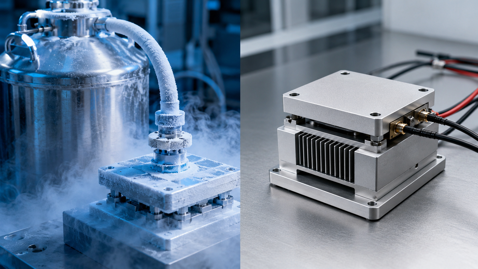
1. How LN₂ Cooling Works — and What It Costs
Liquid nitrogen is cold by chemistry: it boils at −195.8 °C, and every gram that evaporates carries away its latent heat. An LN₂-cooled stage plumbs that fact to the sample platform — by pumping liquid through channels, or by cold-finger contact with a reservoir — while a resistive heater works against the cold to hold any setpoint in between. The reach is the headline: sample temperatures down to the −190 °C region, the full deep-cold band where cryogenic materials science lives1, and low enough to matter for superconductivity work in the post-1986 era when transition temperatures crossed the nitrogen line2 — the low-temperature tradition that began with liquefied gases in the first place3. The costs are logistical and physical: a dewar to fill and refill, transfer lines and boil-off, frost management around every cold surface, and the thermal-stress awareness that fast deep cooling demands of samples and hardware alike — the thermal-shock literature is the cautionary canon here4.
2. How Thermoelectric Cooling Works — and Where It Stops
A thermoelectric element is a heat pump with no moving parts: current through semiconductor junctions carries heat from one face to the other (the Peltier effect), so one face chills while the other warms — reverse the current and the faces swap jobs. The physics, materials and engineering limits are classical and well mapped5, and the limits are the point: each stage of a TEC can sustain a finite temperature difference against its heat load, so single-stage devices reach a few tens of degrees below ambient and stacked multi-stage designs push toward the −60 °C region as a technology class — individual product floors differ (single-stage Peltier platforms commonly specify around −25 °C; check each model’s datasheet) — and there, for practical stage purposes, the road ends. Everything else is advantage: no cryogen logistics (the module itself is dry; fans, heat sinks or a chiller handle the hot side), quiet near-vibration-free operation at the module level that suits high-magnification optics, and electronic reversal that makes thermal cycling straightforward — within the limits set by thermal mass, hot-side rejection and controller dynamics — with control loops exploiting the same electrical immediacy to hold tight stability. For device work where the sample itself dissipates power, a TEC can compensate for self-heating within its heat-pumping and rejection capacity — added dissipation reduces the achievable temperature difference6.
3. Head-to-Head: The Honest Table
| Criterion | LN₂ cooling | Thermoelectric (TEC) |
|---|---|---|
| Coldest reach | ≈ −190 °C | ≈ −25 to −60 °C (design-dependent) |
| Consumables | Liquid nitrogen supply & logistics | No cryogen; power & heat rejection still needed (fans/chillers on some systems) |
| Cooling speed at depth | High — cryogen does the work | Moderate; slows near its floor |
| Thermal cycling | Capable, cryogen-hungry | Convenient — within thermal-mass, pumping & rejection limits |
| Vibration & noise | Boil-off and flow can intrude | Quiet at module level (fans/chillers add their own) |
| Frost management | Mandatory discipline | Needed only below dew point |
| System complexity | Dewar, lines, exhaust | Cables and a heat sink |
| Natural home | Deep-cold science; wide-span stages | Near-ambient precision; cycling; optics-critical work |
4. Interactive: The Cooling Race Lab
The simulator below races the two methods to a target of your choosing. Set the goal temperature and watch both cooling curves run: the TEC curve is quick and clean until it flattens against its floor; the LN₂ curve keeps going long after the TEC has surrendered.
The teaching point is the flatline: above roughly −60 °C the two technologies genuinely compete on speed, stability and convenience — below it, within the compact stage classes compared here, deep cryogenic operation generally shifts the choice to LN₂ (closed-cycle and helium systems form other valid categories). Curves, floors and time constants are schematic teaching constructions; real performance is model- and heat-load-specific.
5. Inside the Machines: Why Each Floor Exists
The two floors — −190 for the cryogen, the −60 region for the semiconductor — are not marketing numbers; each is physics, and knowing why builds sound intuition for the whole decision. Liquid nitrogen’s floor is thermodynamic: a boiling liquid pins itself at its boiling point, −195.8 °C at atmospheric pressure, and every gram that evaporates absorbs a fixed latent heat — the stage merely arranges for that absorption to happen where the sample is. The cold is, in effect, purchased in advance at the air-separation plant and delivered as stored refrigeration; the stage’s own job is plumbing and control, which is why LN₂ systems cool fast at depth — the refrigeration capacity is enormous and already paid for. The long low-temperature tradition, from the first liquefaction era onward, is built on exactly this logistics of bottled cold3.
The thermoelectric floor is subtler: a Peltier junction pumps heat in proportion to current, but the same current generates Joule heat inside the element, and heat also leaks backward down the element’s own thermal conductivity from hot face to cold. The sustainable temperature difference is where pumping, self-heating and back-leak balance — a materials-limited ceiling captured in the thermoelectric figure of merit, which rewards semiconductors that conduct electricity well but heat poorly5, a combination nature grants grudgingly because the same lattice carries both currents7. Stacking stages multiplies the achievable ΔT at rapidly diminishing efficiency, which is why multi-stage devices reach the −60 region and then stop economically rather than abruptly. One floor is a property of a molecule; the other is a property of a materials trade-off — and that is why no amount of engineering moves either very far1.
6. Running Costs & Everyday Logistics
Purchase price is the visible cost; the decision-grade numbers are the running ones, and they differ in kind, not just size. The LN₂ column reads like logistics: a supply contract or an in-house generator, dewar rental and refills, transfer-line hardware, boil-off losses that continue whether or not you measure (storage dewars breathe), and the scheduling tax of “is there enough nitrogen for tomorrow’s run?” None of it is difficult — hospitals and universities run LN₂ economies at scale — but it is a standing commitment, and a lab buying its first cryogenic capability should price the routine, not just the stage. Safety practice rides along: oxygen-displacement awareness in small rooms, cryogenic-handling training, and the unglamorous discipline of not sealing a boiling liquid in a closed volume.
The thermoelectric column reads like electronics: electricity, a heat sink or modest recirculating chiller to carry away the pumped-plus-generated heat, and a low logistics burden — no consumables, no deliveries, no morning dewar check. Duty-cycle costs favor the TEC further: it reaches operating temperature in minutes from a cold start, and near-ambient hold power is modest and system-specific — holding a deep temperature difference still draws continuous power and heat rejection — where an LN₂ workflow amortizes fills and cooldown over the session. The honest synthesis is a usage-pattern question. Daily, unpredictable, near-ambient work — the screening lab, the QC bench, the shared instrument — suits the TEC’s zero-logistics profile. Campaign-style deep-cold work — a week of transport measurements, a cryo-microscopy study — suits the cryogen, whose per-run cost shrinks as the campaign lengthens. And a lab already plumbed for nitrogen has, in effect, prepaid the LN₂ column’s fixed costs — which is why the same stage can be the right buy in one building and the wrong one across the street.
A one-paragraph budgeting frame ties the column together. For a candidate stage, sketch three numbers per option: acquisition cost, a realistic annual running figure (nitrogen contract and boil-off on one side; electricity and a chiller’s upkeep on the other), and a usage forecast in sessions per month. Divide and compare cost per session at your cadence, not the brochure’s — the crossover is striking: heavy deep-cold campaigns amortize the cryogen’s logistics into insignificance, while occasional near-ambient work makes every idle dewar-day a surcharge. The exercise takes ten minutes, forces the usage-pattern conversation the decision actually hinges on, and routinely changes which quotation gets signed.
7. The Decision Tree
Q1 — What is your coldest required temperature? Below −60 °C: LN₂, decision over. Between about −25 and −60 °C: TEC is in play if a multi-stage design covers your point with margin; check the specific model’s floor against your heat load. Above −25 °C: TEC is often attractive when payload, atmosphere, cycling and heat rejection fit the system envelope; LN₂ needs a positive reason. Q2 — Will you cycle? Frequent up-down protocols favor TEC’s rapid electrical reversal strongly (sample response remains limited by thermal mass and heat rejection). Q3 — How sensitive are your optics? Vibration-critical high-magnification work leans TEC within its reach. Q4 — What’s your LN₂ situation? A lab with established nitrogen supply pays little for the cryogen route; a lab without one should count the logistics honestly. Q5 — Might your program go colder later? A wide-span LN₂ stage is the future-proof buy; a TEC stage is the perfect-fit buy. Both answers are legitimate — they are answers to different questions.
8. Vibration, Optics & the Third Vote
A third voter sits quietly at the table whenever the microscope’s magnification climbs: mechanical and optical quiet. Thermoelectric stages are solid-state still lifes — no boiling liquid, no flow pulses, no transfer-line tremor — and at high magnification that silence is data quality: sharper long exposures, steadier focus stacks, cleaner digital correlation. The sensitivity of scanned-probe methods makes the point at its extreme — the tunneling microscope’s atomic resolution was, from birth, a triumph of vibration isolation as much as electronics8 — but everyday optical work feels the same physics: full-field imaging and correlation techniques earn their precision only when the scene holds still9. LN₂ systems are not disqualified — well-designed cold stages manage boil-off and decouple flow admirably — but the vibration column belongs in the comparison table, and for optics-critical near-ambient work it often casts the deciding vote.
The optical ledger has two further lines. Frost exposure differs by duty: a TEC stage spends most of its life above the dew point and visits condensation territory briefly; an LN₂ stage lives below it, making purge discipline a running cost of image quality, not just of sample safety — every minute of imperfect purge is a minute of window haze. Thermal gradients bend light: steep temperature differences across the optical path add subtle refractive gradients (schlieren) that soften high-NA imaging; the milder gradients of near-ambient TEC operation are gentler on wavefronts than the steep cold plumes of a cryogen system working hard. None of these lines overturns the reach argument — below −60 °C the cryogen stands alone — but within the overlap zone, where both machines can do the job, the microscope usually prefers the quieter one.
9. Edge Cases & Hybrids
Three refinements complete the picture. Combined stages: wide-range LN₂-cooled, resistively heated designs span from deep cold to serious heat in one unit — the span-everything workhorses of the temperature-ranges map — at the price of carrying cryogen logistics even on warm days. TEC as precision trim: thermoelectric elements excel not only as primary coolers but as fine-control layers, exploiting their electrical immediacy for tight stability near ambient — the regime where ±0.1 °C specifications do their best work. The frost frontier: whichever method takes you below the local dew point inherits the same enemy — condensation and frost on sample and windows — and the same remedy of dry purge and sealed chambers; the cryogenic-microscopy chapter treats that discipline in full. Traceable temperature accuracy, as everywhere in this hub, rides on the calibration chain regardless of which machine makes the cold10.
10. FAQ: Choosing a Cooling Method
11. Keep Exploring the InSitu Pro™ Knowledge Hub
This article is the cold-side technology chapter of the InSitu Pro™ knowledge hub. To keep going:
- Temperature ranges explained — the full −190 to 1700 °C map this decision lives on.
- Cryogenic microscopy below −100 °C — the science waiting on the LN₂ side.
- Thermal stability & ramp rates — what the control loop does with the cold.
- The theory-guide pillar — heat flow, lag and control in full.
- How to choose an in-situ stage — where this decision slots into the five steps.
- All InSitu Pro™ stages — LN₂, TEC and combined configurations; or use the stage selector.
References
This article compares LN₂ and thermoelectric cooling in general terms. Achievable floors, cooling rates, stability figures and cycling performance are model-, design- and heat-load-specific; consult the applicable product datasheets and validate against your own requirements before purchase or quantitative use. The interactive simulator is a schematic teaching tool with illustrative curves, not performance data for any real stage. Contact ACS Material to match a cooling architecture to your application.