Below −100 °C, materials stop behaving like their room-temperature selves — and often start telling quieter, clearer truths. Thermal vibrations that smear spectra and blur order quiet down; delicate electronic phases that ambient noise destroys emerge and organize; transformations may be kinetically arrested or slowed into observability over the experimental timescale. Cryogenic microscopy — watching samples through a microscope, spectrometer or probe station while an LN₂-cooled stage holds them in the deep-cold band — is the discipline of listening at that temperature. This article makes the scientific case: what physically changes below −100 °C, the three families of phenomena that are especially accessible in this range, and the practical craft — frost, contraction, thermal shock — of working where water vapour and CO₂ frost every unguarded surface, and where, deeper still, the very constituents of air approach their own condensation points (oxygen near −183 °C, nitrogen near −195.8 °C).
1. What Physically Changes Below −100 °C
Temperature is thermal agitation, and removing it changes the rules three ways. Thermal broadening falls: thermal occupation and phonon-related broadening often decrease (detector and electronic noise do not necessarily fall the same way) — lattice vibrations shrink, spectral lines typically sharpen, and signals buried in room-temperature blur become resolvable — the general dividend every cryogenic spectroscopist collects. Energy scales become visible: phenomena whose characteristic energies are small — superconducting gaps, magnetic ordering, subtle structural distortions — are simply erased by ambient thermal energy and reappear only when the sample is colder than they are. Kinetics slow dramatically: thermally activated processes decelerate exponentially, so diffusion, relaxation and transformation slow by orders of magnitude — the physics that lets cold both preserve and reveal. The practical craft of measuring in this regime has its own literature, and it repays reading before the first dewar arrives1.
2. Electronic Order Emerges: The Deep-Cold Headliners
The deep-cold band is where condensed-matter physics keeps its trophies. Superconductivity opened the era — discovered at liquid-helium temperatures in the first golden age of low-temperature physics2 — and the 1986 copper-oxide breakthrough dragged transition temperatures up across the liquid-nitrogen line, transforming LN₂-cooled measurement from a preliminary check into the main event3. Around superconductivity cluster its relatives: metal–insulator transitions, where correlation physics reorganizes conduction itself — framed by the classic Mott analysis4 and mapped across materials families by the modern review literature5 — along with charge and magnetic ordering, and, in clean two-dimensional systems under field, quantized transport phenomena whose discovery reset metrology itself6. In the materials that host them, these states emerge only well below ambient. A cryo-capable stage on a probe station or spectrometer is the entry ticket to all of them.
3. Transport Tells Its Story
Resistance versus temperature is the deep-cold band’s narrative instrument, and cooling is how you make it talk. Metals and semiconductors diverge on the way down — metallic resistance falls as phonon scattering freezes out, semiconductor resistance climbs as carriers freeze onto their donors — and the divergence itself is a classification measurement. Below that first chapter come the finer ones: in disordered systems, conduction crosses into hopping regimes whose signatures — variable-range hopping and the interaction-driven refinements to it — are read directly from the shape of R(T) at low temperature78. The electrical wing of this hub (the R(T) guide and the four-probe/Hall chapter) covers the measurement craft; the point here is motivational: the deep-cold portion of an R(T) curve is where a material’s conduction mechanism signs its name.
4. Interactive: The Cold Landscape Lab
The simulator below rides the thermometer down. Drag the temperature from ambient to −190 °C and watch two archetypal resistance curves diverge — a metal falling, a semiconductor climbing — while the read-out names what each regime unlocks along the way.
The divergence is the lesson: the same cooling run classifies conduction, and the interesting fine structure — transitions, plateaus, hopping curvature — lives disproportionately in the coldest third of the axis, which is exactly the part only an LN₂-class stage reaches. Both curves are schematic archetypes with teaching parameters, not data for any real material.
5. The Deep-Cold Hall of Fame
Deep cold’s résumé is best read as a hall of fame, because an outsized share of condensed-matter’s trophies were won below −100 °C. The Hall effect itself — the sideways voltage a magnetic field extracts from a current — was discovered at room temperature in 18799, but its most profound chapter waited a century for deep cold: in 1980, a cold, clean two-dimensional electron system under field produced Hall resistance quantized so exactly that the effect now anchors the electrical units6. Scanning tunneling microscopy, born in 1982, found its highest form at cryogenic temperatures, where thermal drift and spectral broadening fall away and single atoms sit still enough to be interrogated one by one10. Superconductivity’s modern era — the 1986 copper-oxide breakthrough — specifically moved the drama into liquid-nitrogen reach, making the LN₂-cooled measurement the front row of the field3.
The two-dimensional materials program extended the tradition to the current generation. Graphene’s isolation opened a family of atomically thin systems11 whose intrinsic physics is read at low temperature — suspended graphene’s celebrated carrier mobilities are low-temperature measurements, where phonon scattering quiets enough for the electrons’ true character to show12 — and the semiconducting members of the family, prototyped as transistors, are characterized across cooling curves as standard practice to separate intrinsic transport from thermally activated artifacts13. The pattern across all six entries is identical and is this article’s thesis in historical form: cold did not merely improve these measurements — it was the condition under which the phenomena existed to be measured at all.
6. Freezing States Into View
The third gift of deep cold is stopping time. Because activated kinetics slow exponentially, cooling arrests processes mid-flight: metastable phases that would relax in minutes at ambient can persist for the practical duration of an experiment below −100 °C; solvent and moisture dynamics slow to a crawl; delicate microstructures hold still for long acquisitions. The observational uses follow naturally — cool through a transformation to capture its intermediate stages on the way down; hold at depth to study a frozen state at leisure; rewarm under observation to watch the arrested process resume, now on a timescale the instrument can follow. Combined with the frost-controlled sealed chamber that makes optical access possible, this turns the cryo stage into a device for browsing a material’s kinetic history one temperature at a time.
7. Mounting & Thermal Anchoring at Depth
Between the science and the frost sits an unglamorous discipline that decides whether deep-cold data is quantitative: getting heat out of the sample and knowing you have done so. Anchoring is the first law. At −150 °C, the dominant thermal link between sample and platform is conduction through the mounting interface; a specimen resting loosely on the block is thermally adrift, cooled mostly by whatever gas surrounds it, and can sit many degrees above the platform while the display reads perfectly. Thin, conformal bonding — cryo-compatible grease or adhesive applied sparingly, spring or clamp pressure where chemistry is unwelcome — turns the interface from bottleneck into anchor; the low-temperature measurement literature treats this contact problem as the craft it is1.
Contraction is the second. Sample, adhesive and platform all shrink on cooling, each by its own coefficient, and the differential can debond a joint that was sound at ambient — precisely when you cannot reach in to fix it. The defenses are material choice (bond lines that stay compliant cold), geometry (small bonded areas strain less), and moderated first cooldowns that let stresses relax rather than snap. Verification is the third. A one-time commissioning check — a fine thermocouple or a known transition standard on a dummy sample at the real mounting, in the real purge — measures your platform-to-sample offset across the descent and converts it from unknown to correction. The habit costs an afternoon and upgrades every subsequent cold dataset; the hub’s standing rule — verify at the sample — simply bites hardest where the gradients are steepest.
8. Spectroscopy in the Cold: What Sharpens and Why
Spectroscopists go cold for a specific, calculable reward: linewidth. A Raman or photoluminescence line at room temperature is broadened by the thermal bath — phonon populations shorten excited-state lifetimes, anharmonic interactions smear vibrational energies, and the ensemble averages over a hotter, busier lattice. Cool the sample and the bath quiets: lines narrow, weak features emerge from between collapsed neighbours, and peak positions shift along temperature dependences that are themselves information — the classic Raman studies of semiconductors mapped these shifts and widths into quantitative anharmonicity physics decades ago, making the temperature axis a spectroscopic instrument in its own right14. The craft consequence runs both directions: deep cold typically gives markedly sharper, more resolvable spectra, and the trajectory of a peak on the way down — its shift rate, its narrowing law — identifies and characterizes the modes involved.
Two-dimensional materials turned this old craft into a modern workhorse: graphene’s Raman signature is so temperature-sensitive that its peak positions serve as local thermometers, a dependence calibrated across cooling curves in the foundational measurements of the field15. The generalizable lessons for any cold spectroscopist: acquire the whole descent, not just the endpoints, because the temperature dependence is the analysis; budget laser power doubly, since the same absorbed milliwatts that gently warm an ambient sample can locally erase the cold you paid for; and let the sharpened low-temperature spectrum define your peak model, then carry that model back up the axis — features unresolvable at 20 °C often deconvolve cleanly once their cold positions are known. Sharp spectra are not merely prettier; they are the higher-information version of the same measurement.
9. The Craft: Frost, Shock & Shrink
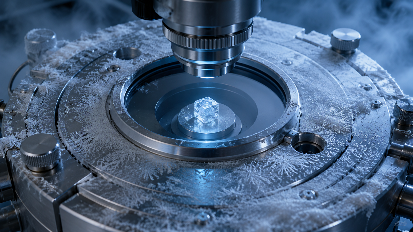
Frost is the defining enemy. Any surface below the local dew point collects condensation, then ice; below −100 °C in ordinary humid laboratory air, an unprotected surface can frost over within minutes, and windows follow. The remedy is architectural — a sealed chamber, dry gas purge, and the discipline of keeping it sealed through the whole cold excursion; the cold outer window surface has its own dew-point management. Thermal shock is the second hazard: plunging brittle samples toward −190 °C imposes transient stresses that can crack them, the classic thermal-stress-resistance problem16 — controlled ramps rather than crash-cooling are the everyday defense. Contraction is the quiet third: sample, adhesive and platform all shrink on cooling, and differential contraction can debond, strain or misalign what was flat and stuck at ambient — mounting choices matter more at −150 °C than anywhere else. And as always, the displayed temperature is the sensor’s, traceable through the calibration chain17; at deep cold, gradients between platform and sample top surface deserve explicit respect. A pocket checklist for the first descent gathers the craft in one breath: dry purge established and the dew point beaten; sensor calibration verified at depth; thermal contraction of sample, adhesive and mounts accounted for; cooling rate chosen with shock in mind; window defogging arranged; and the platform-to-sample offset measured, not assumed.
10. Hardware Notes
The deep-cold band is LN₂ territory by physics — the thermoelectric road ends near −60 °C, as the cooling-methods chapter details — so cryogenic microscopy runs on LN₂-cooled stages: sealed, purge-ready chamber options (configurations vary by model) with optical windows for microscopy and Raman work, and electrically fed-through variants for the transport science of Sections 2–3 on probe stations. Within the InSitu Pro™ family, the wide-span LN₂ stages cover the full descent from ambient heating territory to the −190 °C region in one unit; the selection guide and stage selector match window, chamber and feedthrough options to your instrument, with configuration confirmed at quotation.
11. FAQ: Cryogenic Microscopy
12. Keep Exploring the InSitu Pro™ Knowledge Hub
This article is the deep-cold chapter of the InSitu Pro™ knowledge hub. To keep going:
- LN₂ vs thermoelectric cooling — why this band belongs to the cryogen.
- Temperature ranges explained — the full axis this band anchors.
- Resistance vs temperature: measuring R(T) in-situ — the transport craft for Section 3.
- Four-probe & Hall at variable temperature — deeper into cold transport.
- Variable-temperature Raman — sharpened spectra on the way down.
- All InSitu Pro™ stages — LN₂ configurations for microscopy, Raman and probe work; or use the stage selector.
References
This article discusses cryogenic microscopy in general terms. Achievable temperatures, frost management, thermal-shock tolerance and gradient behaviour are model-, sample- and configuration-specific; validate against the published literature, applicable datasheets and your own measurements before quantitative use. The interactive simulator presents schematic archetype curves with teaching parameters, not data for any real material. Contact ACS Material to configure a cryogenic stage for your instrument and application.