
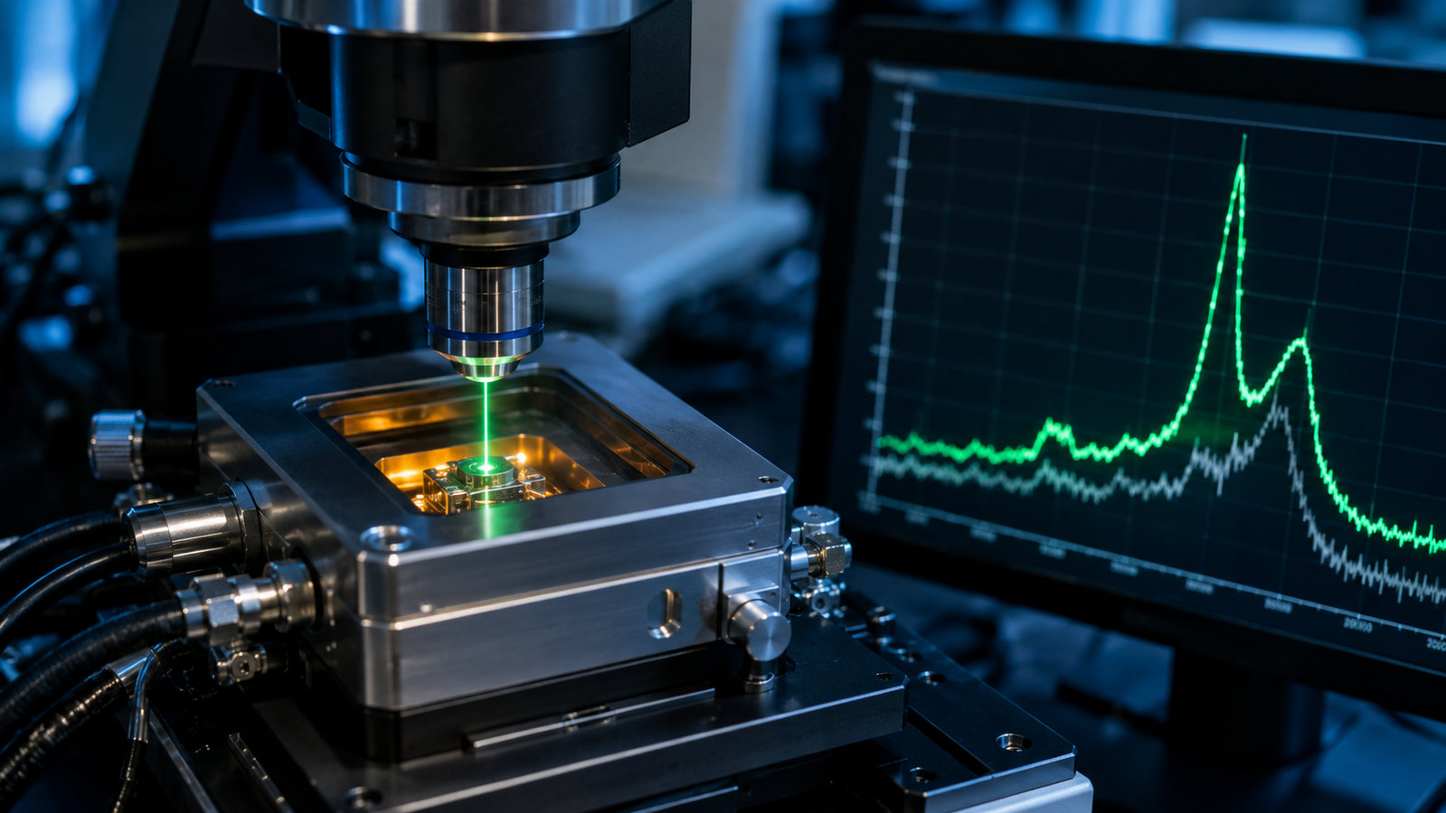
A Raman spectrum is supposed to be a fingerprint — and then you heat the sample, and the fingerprint starts to move. Peaks slide downhill, widths grow, intensities re-balance, and sometimes a whole family of lines vanishes at a phase transition while another is born. None of that is drift or misalignment. It is physics, it is quantitative, and once you learn to read it, a variable-temperature Raman experiment becomes two instruments in one: a structural probe and a built-in thermometer. This guide covers what temperature actually does to a spectrum, the anharmonic physics underneath, how Raman thermometry works, the laser-heating error almost everyone makes once, and what the hardware has to deliver — from cryogenic starts to red-hot finishes.
1. Why Measure Raman as a Function of Temperature?
A single room-temperature spectrum answers one question: what is this material, right now. A temperature series answers better ones. How does the lattice respond to heat? Where exactly does the phase transition sit, and is it sharp or smeared? Does the film relax, crystallize, degrade, or react? Raman is unusually well suited to this interrogation because it is non-contact, often requires relatively little sample preparation — though mounting, surface condition, fluorescence, substrate background, and thermal contact all still matter — works through a window, and reads out vibrational structure that responds to almost every perturbation a material can experience — strain, doping, disorder, fields, and, centrally for this guide, temperature2.
The same qualities make VT-Raman a natural operando probe: because the laser interrogates the working material through the optical port of a sealed stage, spectra can be recorded while a catalyst converts feed gas or a device carries current, tying spectral changes to performance measured at the same moment3. And because vibrational frequencies are exquisitely temperature-sensitive, the spectrum doubles as a thermometer for the exact micron the laser touches — a point we will use, and then warn you about, below.
2. Temperature-Dependent Raman Peak Shift, Broadening & Intensity
Heat a typical crystal and several recurring changes appear in its Raman lines. First, peaks usually shift — most often to lower wavenumber, and to first order roughly linearly, though individual modes can stiffen or move non-monotonically when a specific structural change dominates. The G peak of single-layer graphene moves with a temperature coefficient of about −0.016 cm−1 °C−1; the bilayer is barely different at −0.0154. Few-layer MoS2 plays the same tune in two voices: the in-plane E12g and out-of-plane A1g modes soften at about −1.32 and −1.23 × 10⁻² cm−1 K−1 respectively5, and GaN's zone-centre phonons walk steadily downhill from cryogenic to elevated temperatures6.
Second, peaks typically broaden: the linewidth grows with temperature as phonon lifetimes shorten, a dependence measured carefully in crystals as different as silicon and SnO27. Third, intensities re-balance — most visibly between the Stokes line and its anti-Stokes mirror image, whose ratio climbs with the thermal population of phonons. Fourth, at a phase transition, the symmetry changes and the selection rules change with it: whole sets of lines appear, vanish, or split. Go the other way, toward cryogenic temperatures, and spectra usually get easier to read: cooling suppresses the anharmonic contribution to the linewidth, so features that overlap at room temperature often separate into cleaner, assignable peaks8 — though disorder, strain inhomogeneity, electronic coupling, and phase changes can still set the width you actually observe. Cooling is not just "heating in reverse" experimentally; it is often where the spectroscopy gets easy.
3. The Physics: Anharmonic Phonons and the ω(T) Shift
Why do peaks move at all? In a perfectly harmonic crystal they would not: vibrational frequencies would be constants of the structure. Real interatomic potentials are anharmonic, and anharmonicity has two famous consequences. The lattice expands on heating, which softens the bonds and lowers the frequencies; and phonons interact, so an optical phonon can decay into pairs or triplets of lower-energy phonons — the canonical channel being one optical phonon splitting into two acoustic phonons of half the energy9. The decay rate grows with the thermal population of the daughter phonons, which is why linewidths broaden with temperature.
The classic testbed is silicon. Its single first-order line near 520 cm−1 was tracked from 20 to 770 K in 1970, shift and width together10, and later from 5 to 1400 K, where the high-temperature behaviour revealed that three-phonon decay alone is not enough — four-phonon processes must be included to reproduce the quadratic trend11. A companion analysis separated the two contributions to the shift — the part from thermal expansion and the "pure" anharmonic part from phonon–phonon coupling — showing that both matter and neither can be ignored12. The same framework, population factors and all, carries over to two-dimensional crystals, where anharmonic shift and broadening have been mapped in free-standing graphene sheets13.
For daily lab use the takeaway is compact: over a modest range, ω(T) is nearly linear with a material- and mode-specific slope χ; over a wide range, it curves, following the phonon occupation factor rather than a straight line. Both the slope and the curvature are real material properties — which is exactly what makes them usable as a thermometer, and exactly why the calibration belongs to the material, not to the instrument.
4. Interactive: Watch a Peak Move
The simulator below puts the physics of the last section on screen. It renders the Stokes and anti-Stokes lines of a silicon-like model crystal — a single optical phonon following the three-phonon anharmonic model, with the peak position, linewidth, and Stokes/anti-Stokes intensity ratio all computed live from the occupation factor at your chosen temperature. Drag the temperature from 80 K to 800 K and watch the peak slide and fatten while the anti-Stokes line grows from invisible to prominent; then turn up the model laser power and watch a second, subtler effect: the spot gets locally hotter than the stage setpoint, and the "thermometer" starts reading the error you brought yourself.
5. Raman Thermometry: Peak Shift vs. Anti-Stokes/Stokes Ratio
Within a calibrated, single-phase temperature range, selected peak positions, linewidths, and response-corrected anti-Stokes/Stokes ratios all track temperature well enough to be inverted: measure the spectrum, read the temperature. This is Raman thermometry, and it has two great virtues — it is non-contact, and it reports the temperature of the local optical sampling volume the laser actually interrogates, not of a sensor bolted somewhere nearby. Diamond has been calibrated this way across a wide range using the position of its 1332 cm−1 line14, and in microelectronics, specialized Raman-thermography implementations map the temperature inside working transistors, reaching sub-micron spatial or nanosecond-scale temporal resolution with practical trade-offs among resolution, signal, laser dose, and temperature uncertainty — a mature engineering discipline built on the physics of section 315.
Three practical routes exist, with different trade-offs. The peak-shift thermometer is the most precise per photon but needs a calibrated χ and is confounded by stress (section 7). The linewidth thermometer can be less sensitive than the peak position to a uniform stress-induced shift, but it is not strain-independent — inhomogeneous strain, defects, doping, electron–phonon coupling, and the instrument profile all broaden lines too. The anti-Stokes/Stokes ratio avoids a material-specific frequency coefficient — the ratio follows the Bose–Einstein population, a relationship verified back in the earliest silicon work10 — but it still requires a wavelength-dependent instrument-response correction, adequate anti-Stokes signal, and the assumption of local vibrational equilibrium. Whichever you use, the deeper lesson is one this site keeps returning to: the controller readout and the sample temperature are two different numbers, related by a calibration that is specific to the material, the mounting, and the geometry — the same discipline that in-situ X-ray facilities apply when they calibrate furnaces against a crystallographic transition rather than trusting the thermocouple16. Raman simply lets you carry that discipline in the spectrum itself.
| Method | Main strength | Required calibration | Main limitation |
|---|---|---|---|
| Peak position | Strong signal; easy fitting | Material-, mode- and mounting-specific dω/dT | Stress, doping and phase changes also shift peaks |
| Linewidth | Independent observable of anharmonic decay | Width-vs-temperature calibration; instrument profile | Defects, strain inhomogeneity and coupling also broaden peaks |
| Anti-Stokes/Stokes ratio | No material-specific shift coefficient | Spectral-response correction across both sides | Weak anti-Stokes signal, especially at low temperature |
| Phase-transition marker | Strong fixed-point indicator | Known transition under comparable conditions | Valid only near that transition; hysteresis possible |
No route is universally calibration-free: the best thermometer depends on the material, the Raman mode, the temperature range, the signal level, the strain state, and the optical system.
6. Laser Heating in Raman Spectroscopy: How to Test and Correct It
The laser that excites the spectrum also deposits power into the focal spot, and if the sample conducts heat poorly, the spot runs hotter than the stage — sometimes dramatically. Porous silicon is the cautionary tale: its thermal conductivity is so low that a focused beam of modest power raises the local temperature by hundreds of kelvin, an effect strong enough that it was turned into a measurement method — the laser-induced peak shift itself was used to extract the thermal conductivity17. The same inversion, done deliberately and elegantly, is how the thermal conductivity of suspended single-layer graphene was first measured: ramp the laser power, track the G-peak shift, divide by the independently calibrated temperature coefficient18.
What is a technique in those papers is an error in yours if you ignore it. The defence is a power series: at fixed stage temperature, record spectra at several laser powers and extrapolate the peak position to zero power. If the position depends on power, you are heating the spot; if it does not, you are safe at that power. Run the check on the most thermally fragile point of your temperature range — suspended regions, porous films, polymers, and dark absorbing samples are the usual offenders — and re-run it if you change the objective, since a higher numerical aperture concentrates the same milliwatts into a smaller, hotter spot.
7. Stress vs. Temperature: Untangling Two Shifts
Temperature is not the only thing that moves a Raman peak. Mechanical stress shifts phonon frequencies too — in silicon the effect is strong enough, and well enough calibrated, that micro-Raman is a standard tool for mapping local stress in integrated circuits19. In a variable-temperature experiment the two effects arrive together: heat the sample and the film expands against its substrate, or the clamp, or its own coating, and part of the measured shift is thermally induced strain rather than intrinsic anharmonicity. Supported two-dimensional films are the textbook case — the measured temperature coefficient of graphene grown on copper foil differs from that of transferred or suspended material precisely because the substrate participates in the expansion20.
The practical rules follow. Compare like with like: a χ measured on a suspended flake does not transfer to the same material glued to a stiff substrate. Where the science allows, use the linewidth — broadening tracks temperature but is far less sensitive to strain. And treat thermal expansion itself with respect: it is a material property with real spread, from ordinary positive expansion through near-zero to genuinely negative in ceramics like ZrW2O8, whose lattice contracts smoothly on heating21 — one more reason the calibration belongs to the material, never to the technique.
8. How to Choose a Variable-Temperature Raman Stage
A VT-Raman stage is a small thermal machine that must coexist with a microscope, and the coexistence sets the specification. Many environmental stages seal the sample beneath a removable optical window — open-stage geometries exist too — so the working distance of the objective must clear the window and its frame, which is why long-working-distance objectives are the standard companions. The window must transmit both the excitation laser and the Raman-shifted light with minimal aberration, and it contributes optically in a second way that Raman uniquely cares about: quartz and fused-silica components carry Raman bands and broad background of their own22, with positions that respond to temperature and pressure like any other mode23 — and part of that contribution can land in common fingerprint regions. Treat the window's spectrum as something to be measured and characterized, never assumed negligible: record an empty-stage background with the same laser wavelength, objective, focus, polarization, and a representative stage condition, and re-record it whenever the window, objective, alignment, atmosphere, or temperature regime changes enough to move it.
Beyond optics: temperature stability directly limits how small a χ-based shift you can resolve; drift during a long map smears positions; and the ramp itself matters, because a stage that both heats and cools under the objective lets you close hysteresis loops across a phase transition in a single session rather than a week of remounting. Software completes the machine — a stage that scripts temperature profiles and hands off triggers to the spectrometer turns an afternoon of babysitting into an unattended overnight series.
9. Applications: From 2D Materials to Ferroelectrics
Two-dimensional materials are VT-Raman's home turf: layer number, strain, doping, and thermal transport are all read from the G, 2D, E12g, and A1g families2, and temperature-coefficient measurements underpin the optothermal method that produced thermal-conductivity values for monolayer MoS224 just as they did for graphene. Phase transitions are the second staple: because a structural transition rewrites the selection rules, Raman sees it as lines switching on and off — vanadium dioxide's insulator–metal transition, whose rich monoclinic spectrum collapses in the rutile metal, is the workhorse example, and the hysteresis physics behind it is exactly the territory of our in-situ theory guide. In ferroelectrics, the transition announces itself even more elegantly: a soft mode collapses toward zero frequency as the Curie point approaches, a phenomenon whose experimental mapping is one of light scattering's classic achievements25. Add polymers and pharmaceuticals (melting, crystallization, and polymorph conversion tracked band by band) and operando catalysis, where spectra and conversion are recorded on the same working sample3, and the method's range is clear: anywhere structure changes with temperature, VT-Raman watches it happen.
10. Five Questions Before You Start
11. Stages Built for VT-Raman
The InSitu Pro™ Optical Heating and Cooling Stage ACH600S / ACH400SV is the range's purpose-built platform for exactly the experiments in this guide. Both bodies pair liquid-nitrogen cooling with resistive heating at ±0.1 °C stability, ramp at up to 150 °C min−1 heating and 40 °C min−1 cooling, and run fixed-point, ramp, or fully programmed segment profiles from the supplied control software and LabVIEW VIs / C# SDK — exactly the scripting section 8 recommends. The optics are built for the job: reflection or transmission geometry, a manually removable φ25 × 1 mm quartz top window transmitting 220–2500 nm, just 4.5 mm from window to sample surface, and an ultra-thin 24 mm body the product page notes is compatible with compact optical instruments such as Horiba Raman spectrometers.
- ACH600S — −190 to 600 °C, atmosphere chamber: the broad-range workhorse for VT-Raman in a controlled ambient atmosphere.
- ACH400SV — −190 to 400 °C, vacuum chamber: the same optical-stage format for air-sensitive samples and vacuum-compatible cryogenic work with controlled window defogging.
Around them sits the full InSitu Pro™ heating & cooling range — optical, electrical, mechanical, and special-application stages — matched to experiments in the stage selection guide. Not sure which body fits your microscope and temperature program? The InSitu Pro™ Stage Selector walks you from five questions to a one-click quote.
Q. Which direction do Raman peaks shift on heating?
Almost always to lower wavenumber — the lattice expands and phonon–phonon coupling grows, both of which soften the modes. Exceptions exist (some modes stiffen when a specific structural change dominates), which is precisely why the sign and slope are worth measuring rather than assuming.
Q. How accurate is Raman thermometry?
It depends on the route and the calibration. Peak-shift thermometry can resolve a few kelvin when χ is well calibrated and stress is controlled; the Stokes/anti-Stokes ratio needs less calibration but more signal. In all cases the accuracy belongs to the calibration, not to the technique — a χ from the wrong mounting or the wrong strain state transfers its error directly to your temperature.
Q. How do I know my laser is not heating the sample?
Run a power series: hold the stage temperature fixed, step the laser power, and plot the peak position against power. A slope means self-heating; extrapolate to zero power or reduce power until the slope vanishes. Repeat after changing objectives, and be most suspicious of suspended, porous, polymeric, and strongly absorbing samples.
Q. Can I do Raman through the stage window?
Yes — that is the design intent of an optical stage. Use a long-working-distance objective that clears the window, keep laser power modest, and record an empty-stage background under the same wavelength, objective, focus, and polarization — and repeat it after any change of window, objective, alignment, atmosphere, or temperature regime — so the window's own contribution is characterized before you assign features near it.
Q. Heating stage or cryostat — which do I need?
If the science lives above room temperature only, a heating stage suffices. If peak resolution, low-temperature phases, or full hysteresis loops matter, choose a combined heating-and-cooling stage: sharpened cryogenic spectra make assignments easier, and a single mount can then sweep the entire transition in both directions.
Knowledge Hub & Further Reading
- In-Situ Heating, Cooling & Electrical Stages: A Theory Guide — the physics backbone: phase transitions, hysteresis, and why furnace temperature is not sample temperature.
- InSitu Pro™ Optical Heating & Cooling Stage (ACH600S / ACH400SV) — the product page for the optical stage family this guide's experiments run on.
- In-Situ XRD: Watching Crystal Structure Evolve — the diffraction view of the same transitions: what peak position, width, and intensity report in reciprocal space.
- XRD Stage Windows: 2θ Geometry & Kapton Films — what a window does to a beam, in the X-ray world: absorption, background, and displacement error.
- InSitu Pro™ Stage Selection Guide — match temperature range, atmosphere, and measurement to a specific stage body.
References
Disclaimer: This article is an educational overview of variable-temperature Raman spectroscopy and the InSitu Pro™ optical stages. Temperature coefficients, calibration examples, and model parameters quoted here are representative literature values for specific materials and conditions; real samples vary with strain state, mounting, atmosphere, and history — always calibrate against your own system and refer to product datasheets and SDS documents for guaranteed specifications. The interactive simulator is a schematic teaching tool built on a simplified three-phonon anharmonic model, not a predictive instrument for any specific material or stage.