
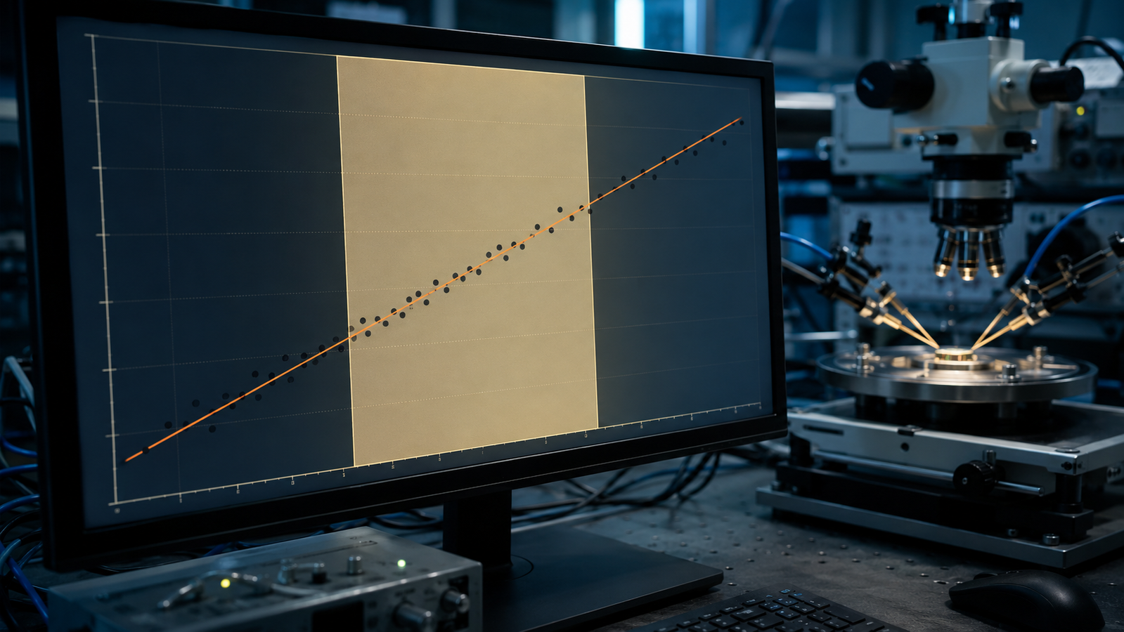
A resistance–temperature curve is raw material, not a result. The result is what you extract from it: a temperature coefficient that qualifies a film for a sensor, an activation energy that identifies a dopant, a critical temperature that goes into a paper, a hopping exponent that diagnoses disorder. Getting from the curve to those numbers is a methodology in its own right — one with well-marked traps, because almost any dataset will yield a straight line on some set of axes, and a straight line is not evidence unless the axes were justified first. The companion overview of variable-temperature electrical probe stages covers the hardware, the transport physics and the classic measurement errors; this article is about the data: how to design the temperature program, what to record, how to fit metals, semiconductors, hopping conductors and superconductors on the right axes, how to budget your errors, and how to report parameters so that someone else could reproduce them.
1. How to Design an R(T) Temperature Program
Every R(T) dataset inherits the quality of its temperature axis, so the program that generates that axis deserves as much design attention as the electrical settings. The axis itself has an official language: practical thermometry worldwide is anchored to the International Temperature Scale of 1990, which defines temperature between fixed points through specified interpolation instruments — the platinum resistance thermometer being the workhorse across exactly the range where in-situ stages live1. A stage controller reports temperature through its sensor, its calibration and its control model; when quantitative transport parameters are the goal, the traceability and uncertainty of that calibration belong in the record. Your job is then to decide how the program moves along the scale.
The first decision is step-and-hold versus continuous ramp. Step-and-hold — move to a setpoint, wait out a stabilization criterion, log the point, move on — gives each datum a defensible temperature at the cost of speed, and is the default whenever the extracted parameter depends on the temperature values themselves: activation energies, TCR, any fit whose x-axis is 1/T. Continuous slow ramps trade per-point accuracy for density, and earn their keep in feature hunting: locating a transition you cannot afford to straddle with coarse steps. Many good campaigns use both — a fast reconnaissance ramp to find the interesting region, then a step-and-hold pass across it.
The second decision is sampling density, and it should not be uniform. An Arrhenius fit wants points spread evenly in 1/T, which means denser temperature spacing at the cold end than the hot end. A superconducting or metal–insulator transition wants dense coverage across a few degrees around the feature and coarse coverage elsewhere. A practical pattern: coarse steps (10–25 °C) across featureless regions, refined steps (0.2–2 °C) across anything with structure, chosen after the reconnaissance pass.
The third decision is direction. Sweep both ways across anything you intend to interpret. Heating and cooling branches that overlay confirm the sample and contacts are stable; branches that separate flag something worth isolating — thermal lag shrinks as you slow the ramp, so rate dependence helps estimate its contribution, though it does not by itself separate equilibrium hysteresis from transformation kinetics or slow chemistry (Section 8).
2. What to Record: the Raw Dataset
The difference between a plot and a dataset is metadata. The 1949 Pearson–Bardeen study that turned silicon’s R(T) into carrier densities, mobilities and ionization energies could do so only because resistivity and Hall data were recorded together, over a documented 87–900 K program, on characterized samples2 — the extraction is only as good as the bookkeeping beneath it.
A minimum recording list for each logged point: temperature (and which sensor reports it), time stamp, resistance, excitation current or voltage and its polarity scheme, and instrument range. Per run: probe layout and spacing, contact verification results at the temperature extremes, atmosphere or vacuum status, ramp/step program, stabilization criterion used, and an event log — every probe re-landing, range change, or interruption. Two habits pay for themselves. First, log time, not just temperature: drift diagnostics live in R(t) at nominally constant T, and you cannot reconstruct them afterwards. Second, record the stabilization criterion itself (“temperature within ±0.2 °C and resistance drift <0.05%/min before logging”) — it belongs in the methods section of whatever the data becomes.
3. Resistance, Sheet Resistance and Resistivity: Which Quantity Are You Fitting?
Before any fitting begins, name the quantity. Resistance R is what the instrument delivers: the terminal voltage over the excitation current, in ohms. Sheet resistance Rs is a thin-film quantity in Ω/□ that exists only relative to a defined two-dimensional measurement geometry. Bulk resistivity ρ additionally requires the sample’s thickness or cross-section and the geometric correction factor appropriate to the probe arrangement — collinear four-point, bar, or van der Pauw — with the standard conversions catalogued in the characterization literature3. Four-terminal sensing suppresses lead and voltage-contact drops; it does not remove the uncertainty contributed by sample dimensions, probe placement, finite contact size or the current distribution. The three quantities are related, not interchangeable.
| Quantity | Symbol | Unit | What it takes |
|---|---|---|---|
| Resistance | R | Ω | The measured voltage over current at the terminals |
| Sheet resistance | Rs | Ω/□ | A defined thin-film measurement geometry |
| Resistivity | ρ | Ω·cm | Resistance plus sample dimensions and the geometric correction factor |
Everything in this article fits R(T), because that is what the stage measures. Whether the extracted temperature dependence transfers cleanly to ρ(T) is a geometry question — answered by the sample’s dimensional stability over the range and by the correction model, not by the quality of the fit.
4. How to Calculate TCR from Resistance vs Temperature
For a metal, the headline parameter is the temperature coefficient of resistance, α = (1/R0)·dR/dT, quoted at a stated reference temperature over a stated interval — both must be reported, because a metal’s R(T) is only locally linear. Near and above room temperature, phonon-limited resistivity rises quasi-linearly and a linear fit over, say, 0–100 °C gives a stable, comparable α; stretch the window toward the cryogenic end and the Bloch–Grüneisen curvature bends the data away from any single line4. A defensible TCR report therefore reads like this: α = 3.4 × 10⁻³ K−1 referenced to 20 °C, linear fit over 0–100 °C, four-probe, terminal resistance — parameter, reference, window, method, quantity. State whether α was computed from terminal resistance, sheet resistance or resistivity: when the sample’s dimensions change with temperature, the resistance TCR and the resistivity TCR are not automatically identical.
Below the linear regime, the informative quantity is the shape: how fast the curve flattens toward its residual floor, which is set by impurity and defect scattering added on top of the phonon term — the additivity known as Matthiessen’s rule. As the companion overview details, a stage reaching 83 K can reveal useful low-temperature curvature and comparative quality trends in some alloys, thin films and high-scattering samples, but does not directly provide the conventional residual-resistance ratio, which is defined against the residual plateau far below — often near 4.2 K — or a separately validated extrapolation5. The honest 83 K deliverables are comparative: R(83 K)/R(300 K) between samples of the same material measured the same way, and the curvature of the approach to the floor. Both rank samples; neither should be relabeled as RRR.
5. Arrhenius Plot for Semiconductor Activation Energy
The workhorse plot for activated transport is ln R against 1/T: an exponentially activated resistance becomes a straight line whose slope, multiplied by the Boltzmann constant, is an energy. The craft is in knowing which energy, over which window.
The slope’s meaning depends on the transport regime and the statistics behind it. In the intrinsic regime, carriers are excited across the gap and the slope delivers approximately Eg/2. In the freeze-out regime of a partially compensated semiconductor the slope tends toward the full donor ionization energy Ed, while in nearly uncompensated material the dilute-ionization statistics give a slope near Ed/2 — the factor-of-two is not a rounding detail but a statement about compensation, and assigning the measured energy to a physical level requires saying which case applies63. This is exactly how the classic silicon analysis proceeded: Pearson and Bardeen extracted donor and acceptor levels not from a single slope but from carrier statistics fitted across regimes2.
Three rules keep an Arrhenius fit honest. First, plot before fitting. Look for straightness over at least one decade of resistance — a fit across a visibly curving stretch returns a number, but the number is a mixture. Second, choose and report the window. An activation energy is only defined together with its fitting range; “Ea = 0.19 eV (fit 140–220 K, ln R vs 1/T, R² = 0.999)” is a result, “Ea = 0.19 eV” alone is an anecdote. Third, respect the bends. A kink between two straight segments usually marks a regime handoff — freeze-out giving way to exhaustion, extrinsic giving way to intrinsic — and each segment gets its own fit and its own interpretation. A continuous downward curvature that never straightens is a different message: no single activation energy describes that interval. Hopping among localized states is one classic explanation7 — Section 6’s territory — but parallel conduction channels, temperature-dependent mobility, contact barriers, compensation and overlapping regimes can all bend the plot the same way, and each deserves a test before a mechanism is declared. What no amount of care can do is make one Arrhenius window summarize a curving dataset faithfully.
6. Variable-Range Hopping: Mott vs Efros–Shklovskii
When the Arrhenius plot curves persistently downward, the standard next hypothesis is variable-range hopping: conduction by phonon-assisted tunneling among localized states, in which the optimal hop trades distance against energy and the effective barrier shrinks with cooling. Mott’s analysis of this optimization gives resistance rising as exp[(T0/T)1/4] in three dimensions — the celebrated T−1/4 law8 — while Efros and Shklovskii showed that electron–electron interactions open a soft Coulomb gap at the Fermi level and bend the exponent to 1/2 at low enough temperature9. The percolation treatment of the random resistor network that underlies these laws was worked out by Ambegaokar, Halperin and Langer10, and the whole framework — including how to tell the regimes apart in real data — is systematized in Shklovskii and Efros’s monograph11.
Dimensionality matters: for ideal Mott hopping the exponent is p = 1/(d + 1) — 1/4 in three dimensions, 1/3 in two, 1/2 in one — so thin-film and 2D-device fits should test 1/3 alongside 1/4. And because Efros–Shklovskii hopping also yields p = 1/2, a fitted half-power is not by itself unique proof of a Coulomb gap11; the assignment needs the dimensionality argument, the temperature window and corroborating dependences to stand together.
The practical fitting problem is that ln R against T−p looks deceptively straight for several values of p at once over a narrow window — Arrhenius (p = 1), Mott (p = 1/4 in 3D, 1/3 in 2D), Efros–Shklovskii (p = 1/2) can all “fit” two decades of data. Two defences: range — a hopping exponent claimed from less than two to three decades of resistance change is weak evidence; and the local-slope test — compute the logarithmic derivative w(T) = −d(ln R)/d(ln T) numerically from the data and plot ln w against ln T: activated and hopping laws each produce a straight line whose slope reveals p directly, without assuming it11. It is the difference between testing a hypothesis and decorating one. Report the exponent with its confidence range, the temperature window, and the diagnostic used — and resist the temptation to promote a fitted p into a mechanism without corroborating evidence such as field or density dependence.
7. Superconducting Tc: Onset, Midpoint & Zero Resistance
A superconducting transition is not a point; it is a curve segment, and “Tc” means nothing until you say which feature of that segment you measured. The standard vocabulary: the onset, where resistance first departs from the extrapolated normal-state line; the midpoint, where R falls to 50% of the normal-state value; the zero-resistance temperature, where R drops below your noise floor; and the transition width, often reported as the 10–90% interval. These are reporting conventions rather than universal definitions — which is exactly why the criterion must travel with the number. In a sharp, homogeneous film these cluster within a fraction of a kelvin; in granular, inhomogeneous or stressed samples they can spread over many kelvin, and the spread is itself diagnostic. A defensible report names the criterion: “Tc(midpoint) = 91.2 K, width (10–90%) = 1.8 K, at 10 μA, zero applied field, cooling branch” — because the historic Y–Ba–Cu–O discovery data themselves show exactly this anatomy, an onset above 90 K with zero resistance settling lower12.
The excitation current belongs in the report because it moves the curve: superconductivity is a critical phenomenon in current as well as temperature, and a too-large measurement current depresses the apparent zero-resistance point and broadens the foot of the transition. The practical check is the same one used throughout low-level transport — repeat the transition at two or three currents and keep the value only when it has stopped moving5. And as the companion overview cautions for 83 K-class stages: crossing the transition of an optimally oxygenated YBCO-family sample is realistic, but whether a stable zero-resistance floor appears by 83 K depends on oxygen content, granularity, current and the true sample temperature — report what the data show, not what the phase diagram promises.
8. R(T) Hysteresis, Thermal Lag and Rate Dependence
Phase transitions announce themselves in R(T) as steps, kinks or loops, and the loop is where method matters most. Vanadium dioxide is the canonical classroom: an insulator–metal transition near 68 °C with a resistance change of several orders of magnitude13, showing a genuine thermal hysteresis between heating and cooling branches — one member of the broad family of correlation-driven metal–insulator transitions surveyed by Imada, Fujimori and Tokura14.
The measurement question is always: how much of the loop is the sample, and how much is the instrument? Thermal lag mimics hysteresis — the sample trails the sensor on every ramp, displacing the heating branch upward in temperature and the cooling branch downward. Rate dependence is the first probe: repeat the loop at two or three ramp rates and extrapolate the branch separation toward zero rate to estimate the lag contribution. A loop that collapses under the extrapolation was lag; one that survives is evidence of material behaviour — but not yet proof of equilibrium hysteresis, because transformation kinetics, incomplete equilibration, contact drift, first-cycle training and slow irreversible chemistry can all sustain rate-robust loops, and a genuine first-order transition’s loop can itself change with ramp rate. Corroborate with equilibrated step-and-hold points on both branches and repeated thermal cycles before the loop is called thermodynamic. For locating the transition temperature itself, the derivative is sharper than the curve: dR/dT (or d(ln R)/dT for multi-decade transitions) peaks at the steepest point of each branch, and the peak positions — quoted per branch, per rate, with the smoothing and differentiation method documented, since derivative peaks move with the filter, the point spacing and the noise — are cleaner coordinates than any eyeballed midpoint. The companion overview’s broader rule applies here: an electrical anomaly alone is a clue, not unique proof of a thermodynamic transition — where possible, correlate it with a structural or optical signature on the same stage.
9. Interactive: The Arrhenius Fitting Lab
The simulator below turns Section 5 into a hands-on exercise. It generates a synthetic R(T) dataset from the same illustrative semiconductor model used in the companion overview — a 1.12 eV gap with a 0.16 eV donor level — sampled across the stage range with realistic measurement noise, and plots it on Arrhenius axes (ln R against 1000/T). Drag the two window handles to choose which temperature range the straight-line fit uses; the readout reports the apparent activation energy from the slope, the fit quality, and which transport regimes your window actually spans. Regenerate the noise to see how stable your fitted energy is against a fresh realization of the same experiment.
The lesson the lab is built to teach: the fitted energy is only meaningful when the window sits inside a single regime. Park the window in the low-temperature freeze-out segment and the slope returns roughly half the donor energy (≈0.07 eV once the small power-law prefactor is folded in), as dilute-ionization statistics dictate for this nearly uncompensated model; park it in the high-temperature intrinsic segment and it returns a slope approaching half the gap (≈0.51–0.53 eV in the hottest windows, climbing toward Eg/2 = 0.56 eV as the extrinsic remnant fades); straddle the exhaustion plateau between them and it returns a smooth, publishable-looking, physically meaningless mixture. The noise button makes the second point: a well-placed window returns the same energy on every regeneration, while a marginal window scatters — fit stability under resampling is a cheap, powerful honesty check — against the imposed random noise only; systematic temperature offsets, contact drift and model bias are untouched by regeneration. Both parameters and both lessons are illustrative; real samples add compensation, parallel channels and contact effects on top.
10. R(T) Error Budget and Measurement Uncertainty
Every extracted parameter inherits errors from two axes, and it pays to know which axis dominates before polishing the other.
The temperature axis. Three layers: sensor calibration against the practical scale1; the sample–stage offset, which depends on mounting, atmosphere and dissipation and must be validated rather than assumed; and dynamic lag during ramps. For activation energies the leverage is multiplicative: the fitted slope goes as 1/T, so for a narrow window and a small common offset δT the extracted energy shifts by roughly the fraction 2δT/T — a 2 K offset around 200 K is already a 2% energy error before anything electrical goes wrong. Treat that as a local estimate: across broad spans, under thermal gradients, or with nonlinear sensor errors, propagate the uncertainty through the full fitting model instead. For transition temperatures the error is direct: whatever the offset is at Tc, that is the error bar floor.
The resistance axis. The residual thermoelectric offset that survives current reversal — the drifting component — sets a voltage floor rooted in the same Seebeck physics that thermoelectric materials exploit deliberately1516. Self-heating converts excitation into a hidden temperature error, worst in small structures where dissipated power concentrates17. Contact behaviour drifts with temperature — a junction that was ohmic warm can turn rectifying cold18 — which is why contact I–V checks belong at the extremes of the range, not just the start. And the sample’s environment writes itself into the curve: suspended-graphene work showed that removing substrate disorder and charged-impurity scattering reveals a strong intrinsic temperature dependence tied to acoustic-phonon scattering19 — the corollary being that supported devices can carry additional substrate-, interface- and process-dependent scattering channels deserving separate evaluation — and hot oxidative exposure alters the sample mid-run20 — an R(T) sweep that chemically edits its own sample yields an irreproducible fit no statistics can rescue.
The budget exercise itself is short: list the terms, estimate each in the units of the final parameter, and spend effort on the biggest one. A typical in-situ Arrhenius fit is limited by the sample–stage offset; a typical Tc report by the criterion choice and current; a typical TCR by the fitting window definition. Precision beyond the dominant systematic is decoration.
11. A Fitting Protocol: From Curve to Reported Parameter
1. Plot first, on more than one set of axes. R vs T, ln R vs 1/T, and — if hopping is plausible — the local-slope diagnostic of Section 5. Let the data nominate the model before any fit runs.
2. Choose the model with a reason. Metallic quasi-linear, activated, hopping, transition — each has a signature shape and a justified axis. A model chosen because “the line looked straight” is a hypothesis, not a conclusion.
3. Define the window before reading the answer. Select the fitting range from the shape (straightness, regime boundaries), not from where the fit returns the number you hoped for. Document the window.
4. Fit, then look at residuals, not just R². Structured residuals — a bow, a kink — mean the model or window is wrong even when R² is seductive. Over narrow windows nearly everything correlates.
5. Stress the fit. Shrink and shift the window; refit the heating and cooling branches separately; if the simulator lesson applies, resample or re-measure and watch the parameter’s stability. Standard low-temperature practice treats a parameter that moves under these perturbations as unfinished business5.
6. Report the triple. Value, window, model — plus the criterion (for Tc), the excitation (always), and the temperature-axis validation. The test of a good report is that a stranger with your raw data reaches your number without asking you anything.
The whole article, at a glance:
| Measurement goal | Recommended plot | Extracted quantity | Main caution |
|---|---|---|---|
| Metallic TCR | R (or ρ) vs T | α + reference T + window | Confirm the linear range; state which quantity α refers to |
| Semiconductor activation | ln R vs 1/T | Ea (value, window, model) | Fit one justified regime; mind the statistics factor |
| Mott VRH | ln R vs T−1/4 or T−1/3 | T0, exponent p | Dimensionality must be justified; use the local-slope test |
| Efros–Shklovskii VRH | ln R vs T−1/2 | TES | p = 1/2 alone is not unique proof of a Coulomb gap |
| Superconducting transition | R vs T | Tc onset / midpoint / zero-R + width | Report criterion, current, field and branch |
| Hysteretic transition | Heating/cooling overlay | Branch temperatures, dR/dT peaks | Separate lag, kinetics and irreversibility before calling it equilibrium |
12. Hardware Notes for Method People
Methodology quietly assumes hardware. Step-and-hold logic assumes a stage whose stability makes the wait criterion meaningful — the InSitu Pro™ AECH600S / AECH400SV electrical stage holds ±0.1 °C across −190 °C to 600 °C (air chamber) or −190 °C to 400 °C (vacuum) — the published stage stability that lets a “within-band and drift-free” criterion converge at all. Stage stability is not sample accuracy: the sample–stage offset, equilibration time and self-heating of Section 10 still need validating for the actual mounting and atmosphere. Four-probe sensing is assumed throughout this article; the stage supplies four individually positionable probes with BNC feedthroughs, with collinear, van der Pauw and Hall-bar geometries treated in the dedicated four-probe & Hall guide. Atmosphere choices — and their quotation-level boundaries — are likewise covered there, along with the full electrical stage family from LN₂-cooled platforms to 1500 °C resistivity configurations.
- Electrical Heating & Cooling Stage (AECH600S / AECH400SV) — the ±0.1 °C four-probe platform whose stability underwrites the step-and-hold protocols in this article.
- Variable-temperature electrical probe stages: the overview — hardware anatomy, transport physics, contact behaviour, measurement pitfalls and model selection across the whole electrical family.
- All InSitu Pro™ electrical stages — the complete electrical-application line; or let the interactive stage selector match your experiment to a configuration.
13. FAQ: R(T) Measurement and Fitting
14. Keep Exploring the InSitu Pro™ Knowledge Hub
This article is part of the InSitu Pro™ knowledge hub on temperature-controlled, atmosphere-controlled characterization. To keep going:
- In-situ heating, cooling & electrical stages: a theory guide — the pillar article on how temperature-controlled stages work, from heater physics to thermal lag.
- In-situ electrical probe stages: variable-temperature transport — the companion overview: hardware anatomy, transport physics, contacts, pitfalls and stage selection.
- Four-probe & Hall measurements at variable temperature — collinear, van der Pauw and Hall-bar geometries, field reversal and carrier extraction: the geometry companion to this article.
- In-situ oxidation studies by optical microscopy — the chemistry that can rewrite a sample mid-sweep, treated as the signal on the same stage family.
- Variable-temperature Raman spectroscopy — the vibrational-spectroscopy complement on the same temperature axis.
- How to choose an in-situ heating & cooling stage — the five-step selection guide with interactive simulators.
References
This article discusses R(T) measurement methodology — temperature programs, fitting models, parameter extraction and error budgeting — in general terms. Activation energies, hopping exponents, transition temperatures and the regime boundaries between them are idealized and material-, doping-, geometry- and instrument-dependent; real behaviour varies with sample quality, contacts, wiring and configuration, and should be confirmed against the published literature, your own calibrations and the manufacturer’s datasheets before quantitative use. The interactive simulator is a schematic teaching tool — its dataset is synthetic, generated from an illustrative model with stated parameters and artificial noise — and is not a substitute for measured transport data.