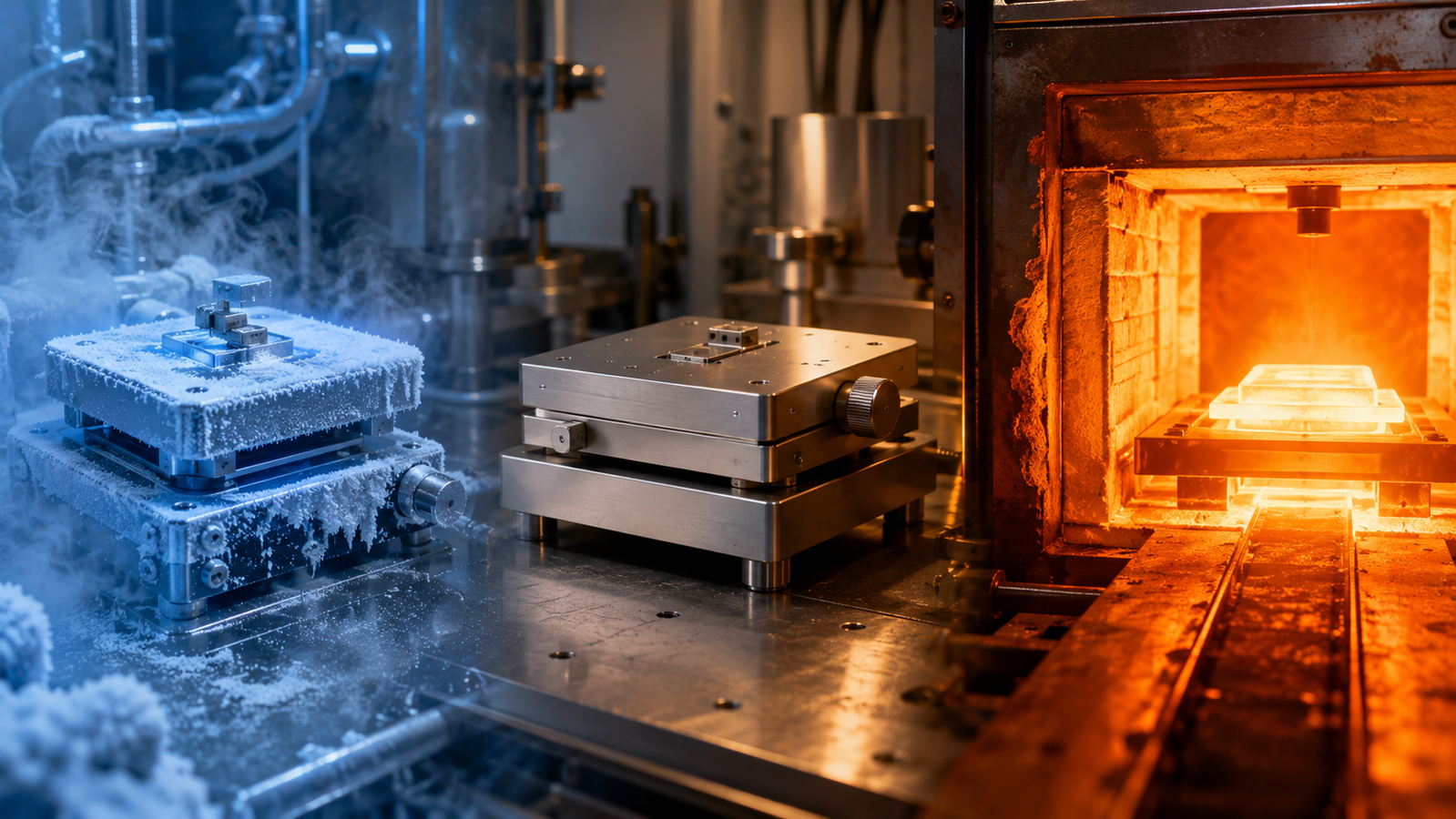
Nearly two thousand degrees separate the coldest LN₂-cooled stages in this family from the hottest — from liquid-nitrogen territory near −190 °C to furnace heads beyond 1500 °C — and no single stage covers the span. That is not a product limitation; it is physics. Different bands of the temperature axis are reached by different machinery, host different phenomena, and impose different engineering compromises. This article is the map: a walk up the axis from the cryogenic floor to the furnace ceiling, what science lives in each band, which cooling and heating technologies serve it, and how to read your own experiment’s position on the map before choosing hardware.
1. −190 °C: The Cryogenic Floor
The bottom of the practical range for LN₂-cooled stage families is set by a substance, not a specification: liquid nitrogen boils at −195.8 °C, and LN₂-cooled stages work a few degrees above it. The science down here is disproportionately fundamental. Low temperature is where thermal noise quiets and delicate electronic order emerges — superconductivity was discovered at liquid-helium temperatures in 19111, and the copper-oxide revolution of 1986 pulled transition temperatures up toward — and eventually past — the liquid-nitrogen line, which is precisely what made LN₂-cooled measurement scientifically electric2. It is also where materials engineering gets serious about cold: cryogenic embrittlement, low-temperature service properties and the whole discipline of measurement at deep cold, codified in the experimental-techniques literature3. The engineering price of the band: LN₂ logistics, condensation and frost management, and thermal-shock-conscious design.
2. −60 °C to Ambient: Thermoelectric Territory
Between deep cryogenics and room temperature runs a band served by an entirely different machine: the thermoelectric (Peltier) element, a solid-state heat pump with no cryogen handling — the hot side still needs adequate heat rejection (fan, heat sink, water loop or chiller) — and superb bidirectional control, whose physics and practical limits the thermoelectric literature lays out4. Single- and multi-stage TEC stages typically reach a few tens of degrees below ambient — the −25 to −60 °C region depending on design and heat load. The science of the band is everyday cold: freeze–thaw and ice nucleation, liquid crystals and soft matter, biological and pharmaceutical stability, condensation studies, and precision temperature-cycling of devices. Because TEC elements reverse by polarity, this is also the natural home of tight thermal cycling protocols. The companion article on LN₂ versus thermoelectric cooling turns this band boundary into a decision tree.
3. Ambient to ~350 °C: The Workhorse Band
The band above room temperature is where most of applied materials science actually happens, and resistive heating serves it simply and well. Polymers melt and crystallize here; pharmaceuticals run their thermal events; solders reflow; water leaves hydrates; solvents and volatiles depart; moderate annealing and aging proceed. It is also where an astonishing amount of correlated-electron physics turns out to live at convenient temperatures — the canonical vanadium dioxide metal–insulator transition sits near 68 °C, within reach of the gentlest heater5. Engineering in this band is friendly: standard windows, standard seals, modest gradients — which is why the workhorse stages of optical, Raman and electrical work cluster here, and why ±0.1 °C stability specifications are both achievable and scientifically meaningful (the stability guide in this hub explains what that number buys).
4. Interactive: The Temperature Atlas
The simulator below is the article in one control: drag the cursor along the full −190 to 1700 °C axis and watch the technology band, the characteristic phenomena and the engineering notes update at every stop.
Use it as a planning tool in miniature: place your experiment’s hottest and coldest required points on the axis, and the bands they fall in tell you which cooling/heating technologies — and therefore which stage classes — are in play. The atlas is schematic and representative, not exhaustive; band edges in real products vary by model and configuration.
5. 350–600 °C and Beyond: The High-Temperature Band
Above roughly 350 °C the experiment changes character. For many bulk metals, oxidation in air stops being a nuisance and becomes a dominant process — atmosphere control graduates from option to necessity (oxidation-prone systems — thin films, fine powders, copper, reactive alloys — cross that line far earlier). Radiation joins conduction and convection as a serious heat-transfer channel, gradients steepen, and window and seal materials start earning their specifications. The science of the band is correspondingly muscular: oxidation and corrosion kinetics as deliberate studies, phase transformations in steels and alloys, decomposition and calcination, glass transitions of inorganic systems, thermoelectric and functional materials at operating temperature. Stage design responds visibly — water-cooled bodies, radiation shields, high-temperature window materials — and the specification sheet grows an atmosphere column.
6. 1000–1700 °C: Furnace Class
The top of the range belongs to purpose-built furnace heads, most at home on X-ray diffractometers where the science demands them. This is ceramic country: sintering — whose classical kinetics were mapped in the founding literature of the field67 — along with solid-state synthesis, refractory phase equilibria, melt studies and the upper reaches of metallurgy. Everything is harder here: sample containment and reaction with holders, thermocouple degradation and calibration at the edge of the practical scale8, radiation-dominated gradients, and optics that must survive facing a white-hot cavity. The synchrotron and furnace chapters of this hub’s diffraction wing cover the craft; for the map’s purposes, the message is simpler — the 1000+ band exists, is served by dedicated hardware, and is where ceramics and refractories do their in-situ science.
7. A Walk Through the Bands: Representative Experiments
The atlas earns its keep when each band is populated with real experiments, so here is the walk, cold end first. In the LN₂ band, the marquee measurement is the superconducting transition itself — resistance collapsing to zero on cooling — joined by the whole repertoire of low-temperature transport: carrier freeze-out, hopping-conduction curvature, and, in clean two-dimensional systems under magnetic field, the quantized Hall plateaus whose discovery reset electrical metrology9. In thermoelectric territory, the everyday sciences of cold: ice nucleation and freeze–thaw cycling, condensation and frost-point studies, the cold-chain stability of biologics and formulated drugs, and the sub-ambient endotherms — freezing water, glass transitions of frozen solutions — on which pharmaceutical development leans10.
In the workhorse heating band, polymers own the stage: isothermal crystallization runs at a series of undercoolings, spherulite growth-rate measurements under the polarizing microscope — the founding craft of polymer morphology11 — alongside pharmaceutical melt-and-recrystallize screens, solder reflow profiling, and epoxy cure monitoring. In the high-temperature band, oxidation kinetics graduate to deliberate studies, steels run their transformation diagrams, and thermal-shock behaviour — the resistance of brittle materials to sudden temperature change — becomes a quantitative subject with its own classical framework12. In furnace class, sintering necks grow between ceramic particles pattern by pattern, solid-state syntheses are followed reflection by reflection, and the exotic corners open: materials with negative thermal expansion contracting measurably, visibly, as the furnace climbs13. One axis; a different science every few hundred degrees.
8. Matching Range to Instrument & Sample
Range questions never travel alone — the instrument and the sample each cast a vote. The instrument’s vote: optical microscopy and Raman spectroscopy travel widely across the axis, though the ride is not free: window materials, working distance, numerical aperture, thermal radiation at the hot end, sample emission and detector response all take their cuts, and working distance shrinks as insulation thickens, so deep-cold and furnace-class stages are engineered specifically to keep the sample close to short-working-distance optics. X-ray diffraction tolerates wider gaps and hotter chambers — which is why the 1000+ band is diffraction country — while electrical probing adds feedthrough and contact-metallurgy constraints that tighten as temperatures leave the workhorse band in either direction. Matching is therefore two-sided: the stage must reach your temperatures and present your instrument with a geometry it can use; the instrument-specific chapters of this hub carry those negotiations in detail.
The sample’s vote: thermal mass sets how faithfully a specimen follows the program (a massive mount lags a fast ramp everywhere on the axis, but the penalty grows where radiation dominates); volatility caps the hot end for organics and hydrates long before the stage’s limit does; and thermal-expansion mismatch between sample, adhesive and platform stresses mounts hardest at the axis’s extremes. A practical planning habit ties the three votes together: write down the coldest and hottest points the science requires, subtract the temperatures the sample can survive, and check the remainder against what the instrument’s geometry permits — the intersection, not the stage catalogue, is your true operating window, and the selection guide in this hub is built to walk exactly that intersection.
9. The Overlap Zones: Where Bands Meet
Band edges here are representative planning bands in this product-and-technology map, not universal physical thresholds — and they are where the interesting engineering lives, and three overlap zones deserve a planner’s respect. The −60 frontier is the LN₂/TEC handover: within roughly −25 to −60 °C both technologies genuinely compete, and the tie-breakers are workflow rather than physics — cycling frequency, vibration sensitivity, nitrogen logistics — the full decision tree of the cooling-methods chapter. Buy for the coldest point you will actually use, not the coldest you can imagine; the zone rewards honesty. The 350 frontier is where atmosphere graduates from accessory to necessity: below it, oxidation is slow enough for many bulk metals that air can often be tolerated — though thin films, nanoparticles, copper and reactive alloys oxidize far lower, and long exposures accumulate; above it, most metals scale visibly on experimental timescales and every heated experiment silently becomes two unless the chamber says otherwise. Stages that straddle this line earn their sealed-chamber options, and protocols that cross it mid-run should decide the atmosphere question before the ramp, not during.
The 1000 frontier is the construction handover from stage to furnace head: radiation now dominates heat transfer, sample–holder chemistry joins the error budget, and the hardware idiom changes from “chamber on a microscope” to “furnace on a diffractometer.” Experiments living just below the line can often stay in friendlier hardware by protocol design; experiments genuinely above it should embrace furnace-class engineering rather than stretch a mid-range stage past its dignity. The general craft of the zones is the same in all three: a requirement sitting near an edge costs disproportionately, because it forces the compromises of the harder band while using little of its reach — so interrogate edge-hugging requirements twice (is −70 truly needed, or is −55 the science?), and when the answer is genuinely “yes, past the edge,” cross it wholeheartedly with hardware built for the far side.
10. Reading the Map for Your Experiment
Three steps turn the map into a shortlist. Fix your endpoints: the coldest and hottest temperatures the science genuinely requires — with a margin, but an honest one, since range costs money and compromise at both ends. Read the bands: endpoints below −60 °C point to LN₂; a cold end within −25 to −60 °C opens the thermoelectric option; a hot end above ~350 °C raises the atmosphere question; above ~1000 °C you are shopping furnace heads. Check the crossings: experiments spanning bands (a −150 to +600 °C study, say) need combined-technology stages, which exist and are specified exactly for this. Then hand the endpoints to the five-step selection guide or the interactive stage selector — range is the selector’s first question — and browse the InSitu Pro™ family with the map in hand: the catalogue is organized along exactly this axis.
11. FAQ: Temperature Ranges
12. Keep Exploring the InSitu Pro™ Knowledge Hub
This article is the axis map of the InSitu Pro™ knowledge hub. To keep going:
- LN₂ vs thermoelectric cooling — the cold-side technology decision in full.
- Cryogenic microscopy below −100 °C — the science of the deep-cold band.
- Thermal stability & ramp rates — what ±0.1 °C buys across every band.
- Synchrotron in-situ furnaces — the top of the axis at full flux.
- The theory-guide pillar — how control works at any temperature.
- All InSitu Pro™ stages — the family, organized along this axis; or use the stage selector.
References
This article maps in-situ stage temperature ranges in general terms. Band edges, achievable limits, stability figures and atmosphere requirements are model- and configuration-specific; consult the applicable product datasheets and validate against your own instruments before quantitative use. The interactive atlas is a schematic teaching tool, not a specification document. Contact ACS Material to match your experiment’s endpoints to a specific stage configuration.