
Real-time PCR reports each reaction as a cycle number: the earlier the fluorescence rises above a set threshold, the more template the reaction started with [1]. That number is commonly called the cycle threshold (Ct) or quantification cycle (Cq); MIQE uses Cq terminology [2][3]. A qPCR efficiency calculation turns a dilution series into a standard curve, and the slope of that curve shows how close each cycle comes to a perfect doubling. This guide covers Ct value meaning, how to build and read a qPCR standard curve, why an amplification efficiency of 90–110% is the usual working window, when ΔΔCt is safe, melt curves, and what the instrument contributes. For where qPCR sits in the wider bench workflow, see From Extraction to Gel Viewing: A Molecular Biology Bench Workflow with PCR, qPCR and Electrophoresis.
Quick answer:
- A Ct value is analysis-dependent: it shifts with baseline and threshold settings. Compare raw Ct values most confidently within the same assay and run; for between-run comparisons, keep analysis consistent and use inter-run calibrators rather than treating raw Ct values as absolute [3–5].
- Efficiency comes from the slope: plot Ct against log10 input for a 10-fold dilution series and calculate E = 10^(−1/slope) − 1; a slope of −3.32 corresponds to about 100% [6][7].
- 90–110% is a working window, not a guarantee: above 110% usually means an artefact (inhibition in the concentrated standards, pipetting error, primer-dimer signal), not a reaction that more than doubles [6][7].
- R² alone does not validate a curve: check the slope, the replicate spread, the no-template control and, for dye-based assays, the melt curve as well [7][8].
- ΔΔCt assumes near-equal efficiencies for the target and reference assays; when they differ, use an efficiency-corrected ratio [9][10].
1. What a Ct Value Means
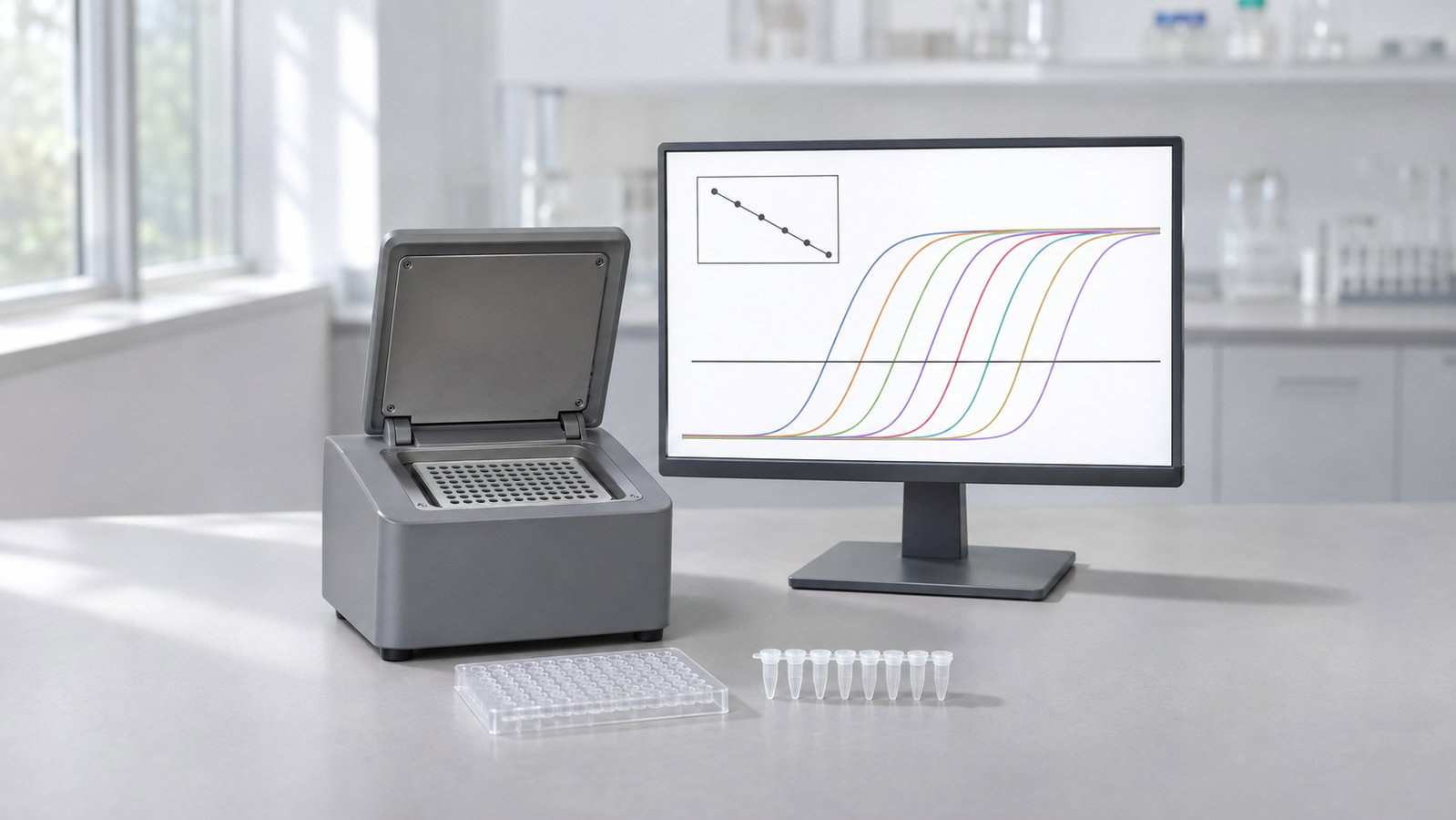
During qPCR, a fluorescent reporter tracks product as it forms. With an intercalating dye such as SYBR Green I, fluorescence rises when the dye binds double-stranded DNA [11]. With a hydrolysis probe, the polymerase's 5′→3′ exonuclease activity cleaves a labelled probe bound to the target, releasing the reporter from its quencher [12][13]. Plotted against cycle number, each reaction gives an amplification curve: a flat baseline, an exponential phase where product roughly doubles each cycle, and a slowing phase that ends in a plateau [14].
The quantification cycle is the fractional cycle at which a curve crosses a fluorescence threshold set above the baseline and within the exponential phase [2]. Because product accumulates exponentially, a reaction with ten times more starting template reaches the threshold about 3.32 cycles earlier when efficiency is close to 100% (2^3.32 ≈ 10) [7]. That is the core of Ct value meaning: a low Ct means more starting template, a high Ct means less.
Two analysis choices move every Ct: the baseline (background subtracted from each curve) and the threshold. Ruijter and colleagues showed that baseline estimation errors feed directly into the observed PCR efficiency and are then propagated exponentially into estimated starting quantities and fold differences [4]. Curve-analysis algorithms also differ in how they place a curve on the cycle axis and determine efficiency [15]. In practice, use a common threshold in the exponential phase for the standards and unknowns being compared, keep analysis settings consistent, and include an inter-run calibrator when results span runs [3][5].
MIQE 2.0 goes further and recommends converting Cq values into efficiency-corrected target quantities and reporting them with prediction intervals, rather than reporting raw Cq values alone [3].
2. Building a qPCR Standard Curve
A qPCR standard curve relates Ct to template input. For absolute quantification, prepare a dilution series from a standard with known copy numbers. For an efficiency or linearity check, a pooled reference sample may also be serially diluted; if its absolute concentration is unknown, plot Ct against log10 relative concentration (1, 0.1, 0.01) rather than assigning copy numbers. Run each dilution in replicate [3][6][7]. Linear regression gives three numbers:
- Slope: cycles per 10-fold change in input; it carries the efficiency.
- Intercept: the extrapolated Ct for one unit of input on the x-axis scale.
- R²: how closely the points follow a straight line; R² > 0.980 is one commonly cited hallmark of an optimised assay, not a stand-alone pass criterion [7].
For absolute quantification, interpolate an unknown's Ct through the fitted line to estimate copy number, provided the standard has a known quantity and the unknown lies within the validated linear range [2][3][6]. For efficiency, the slope is what matters. Bustin and Huggett recommend at least three replicates and four, ideally five, orders of magnitude of template concentration [7]. Svec and colleagues recommend one robust curve with at least 3–4 replicates per concentration, using larger transfer volumes to reduce sampling error in the dilutions [6]. Use only points within the assay's validated linear range, and report the uncertainty of the efficiency estimate; points outside that range can distort the fitted slope [3][6].
| Input (copies per reaction) | log10 input | Mean Ct |
|---|---|---|
| 100,000 | 5 | 16.21 |
| 10,000 | 4 | 19.42 |
| 1,000 | 3 | 22.97 |
| 100 | 2 | 26.18 |
| 10 | 1 | 29.86 |
Table 1. A hypothetical five-point, 10-fold standard curve.
Calculated illustration, not a specification. Inputs: five made-up mean Ct values for a 10-fold series from 100,000 to 10 copies per reaction, fitted by ordinary least squares. Result: slope −3.406, intercept 33.15, R² 0.9995, efficiency about 96.6%. An unknown with a Ct of 24.00 reads back to about 480 copies on this line. These numbers are not output from any instrument software and are not the performance of any ALab system.
Efficiencies from a dilution series can differ from those of the unknown samples. Ramakers and colleagues proposed fitting the log-linear phase of each amplification curve instead [16], and Tichopad and colleagues described a single-reaction approach [17]; both complement a well-made dilution series.
3. qPCR Efficiency Calculation from the Slope
Amplification efficiency (E) is the fraction of template copied in each cycle: E = 1 means perfect doubling. If every reaction in a series reaches the same threshold, Ct falls by 1/log10(1 + E) cycles for every 10-fold increase in input, which gives the textbook relation [6]:
E = 10^(−1/slope) − 1
For a 10-fold series, a slope of −3.32 corresponds to 100% efficiency [6][7].
| Slope (10-fold series) | Efficiency |
|---|---|
| −3.10 | 110.2% |
| −3.32 | 100.1% |
| −3.58 | 90.3% |
| −3.60 | 89.6% |
Table 2. Slope and efficiency from E = 10^(−1/slope) − 1.
Calculated illustration, not a specification. Inputs: the slopes shown, put through the formula above.
Why 90–110%. Amplification efficiency of 90–110% is a common working window rather than a universal acceptance rule. Svec and colleagues note that a properly designed assay, in the absence of interfering substances, should amplify target DNA with at least 90% efficiency [6]. Bustin and Huggett list 95–105% among the hallmarks of an optimised assay, alongside a linear curve, precise replicates, no primer-dimers and a wide dynamic range [7]. MIQE asks for the efficiency, slope, intercept and dynamic range of each assay to be reported [2].
Above 110% is an artefact, not "extra" amplification. A reaction cannot copy more than every template molecule per cycle. Svec and colleagues identify inhibition as a frequent cause of efficiency estimates above 100%: it is pronounced in the concentrated standards, delays their Ct values, flattens the slope and inflates the calculated efficiency if those points are kept in the fit [6]. Other common causes are dilution and pipetting errors [6] and extra signal from primer-dimer or non-specific product in dye-based assays [7][18]. Below 90%, look at primer design, template secondary structure, reagent concentrations and inhibitors carried over from sample preparation [6][7].
| Input (copies per reaction) | Mean Ct, clean series | Mean Ct, inhibited top standards |
|---|---|---|
| 100,000 | 16.21 | 17.60 |
| 10,000 | 19.42 | 20.40 |
| 1,000 | 22.97 | 22.97 |
| 100 | 26.18 | 26.18 |
| 10 | 29.86 | 29.86 |
| Slope / R² / E | −3.406 / 0.9995 / 96.6% | −3.030 / 0.9948 / 113.8% |
Table 3. Inhibition in the two concentrated standards.
Calculated illustration, not a specification. Inputs: the Table 1 series, with the Ct of the two highest standards delayed to 17.60 and 20.40 to mimic inhibition; all other points unchanged. R² still looks high, yet efficiency is pushed above 110%: R² alone does not validate a standard curve. Check neighbouring-point spacing and replicate spread. Treat delayed top standards as a warning: investigate inhibition and dilution accuracy, repeat or dilute the stock as appropriate, and exclude points only when they are demonstrably outside the validated linear range. Document any exclusions [3][6].
4. ΔΔCt and When It Needs Equal Efficiencies
Relative quantification compares a target gene with a reference gene in a test sample and a calibrator, usually an untreated control. In the comparative Ct method [9][19]:
- ΔCt = Ct(target) − Ct(reference), for each sample.
- ΔΔCt = ΔCt(test) − ΔCt(calibrator).
- Fold change = 2^(−ΔΔCt).
The "2" in that formula assumes both assays double their product every cycle. Livak and Schmittgen presented the method together with its assumptions and a validation step: run target and reference on a dilution series and plot ΔCt against log input; a slope close to zero shows that the two efficiencies are similar [9]. Ramakers and colleagues pointed out that the comparative Ct method assumes 100% efficiency (doubling every cycle), an assumption that real assays do not always meet [16].
| Case | Target efficiency | Reference efficiency | Reported fold change |
|---|---|---|---|
| ΔΔCt (assumes 2.0 per cycle) | 90% | 100% | 9.4 |
| Efficiency-corrected ratio | 90% | 100% | 8.0 |
Table 4. A true 8-fold change read two ways.
Calculated illustration, not a specification. Inputs: a true 8-fold rise in the target, a target assay at 90% efficiency (1.90 per cycle), a reference assay at 100% whose Ct does not change between samples. The target Ct shifts by log(8)/log(1.90) ≈ 3.24 cycles; 2^3.24 reports about 9.4-fold, while 1.90^3.24 returns the true 8.0-fold.
Pfaffl's model calculates the ratio from the efficiencies and Ct differences of target and reference, so unequal efficiencies are handled directly [10]. Normalisation matters as much as efficiency: Vandesompele and colleagues showed that a single reference gene can lead to relatively large errors and validated the geometric mean of several carefully selected reference genes as a normalisation factor [20]. Hellemans and colleagues added inter-run calibration and error propagation for several reference genes [5].
5. Melt Curves for Intercalating-Dye Assays
An intercalating dye reports any double-stranded DNA, including primer-dimer and off-target products [11][18]. A melt curve, run after cycling, checks what was actually amplified. The instrument heats the reactions slowly while reading fluorescence; as the product melts, the dye is released and the signal drops. Plotted as the negative derivative of fluorescence against temperature, each product gives a peak at its melting temperature [8].
Ririe and colleagues showed that melt-curve shape and position depend on the GC/AT ratio, length and sequence of the product, and that products less than 2 °C apart in melting temperature can be distinguished [8]. Look for a single sharp peak in each sample and no product peak in the no-template control (NTC). A single peak is not proof of a single product, so confirm the amplicon on an agarose gel when you first validate an assay; Svec and colleagues, for example, confirmed their products by both melting curve analysis and agarose gel electrophoresis [6]. Wittwer and colleagues noted that non-specific products limit dye detection, and that probes add specificity [18].
6. What the Instrument Contributes
A reliable result has three layers: the assay (primers, template, reagents) [7][21], the analysis (baseline, threshold, efficiency, normalisation) [4][5] and the instrument (temperature control, optics, data handling). Svec and colleagues found that the estimated PCR efficiency varied significantly across six instruments but was reproducibly stable on one platform [6]. Build your standard curves on the instrument you will run the samples on.
When reading a specification, distinguish temperature accuracy from uniformity: the product pages give one accuracy value and specify uniformity at specified test temperatures. The heating/cooling rate is a maximum, not the rate of every step.
| Model | Sample format | Heating temperature range | Accuracy | Uniformity | Max. heating/cooling rate |
|---|---|---|---|---|---|
| Accurate 96 | 96-well format | 4–100 °C | ±0.2 °C | ±0.2 °C at 60 °C; ±0.2 °C at 95 °C | 6.0 °C/s |
| Accurate 16-T | 16 wells; 0.2 mL single tubes or 8-strip tubes | 10–100 °C | ±0.2 °C | ±0.2 °C at 60 °C; ±0.3 °C at 95 °C | 6.0 °C/s |
Table 5. Thermal specifications.
| Model | Channels | Dyes | Detection mode |
|---|---|---|---|
| Accurate 96 4-channel | 4 | FAM/SYBR Green, VIC/HEX, ROX, Cy5 | Time-resolved signal separating technology |
| Accurate 96 6-channel | 6 | FAM/SYBR Green, VIC/HEX, ROX, Cy5, Cy3 | Time-resolved signal separating technology |
| Accurate 16-T 2-channel | 2 | FAM/SYBR, VIC | Linear fast well-by-well scanning |
| Accurate 16-T 4-channel | 4 | FAM/SYBR, VIC, ROX, Cy5 | Linear fast well-by-well scanning |
Table 6. Optical configurations.
How to read the tables:
- Both systems use Peltier thermal cycling and a multi-pixel photon counter detector.
- Wavelengths: the Accurate 96 lists an excitation/detection wavelength range of 455–650 nm / 510–715 nm. That is the overall span of the optics, not the band of any single channel.
- Six channels, five dye groups: the Accurate 96 6-channel configuration lists five dye groups across six channels. Ask ACS Material to confirm the sixth-channel dye assignment when requesting a quotation. Other dyes are not covered by these tables.
- Gradient: the Accurate 96 also lists a temperature gradient setting range of 30–100 °C and a gradient difference setting range of 1–36 °C. Annealing-temperature optimisation before a qPCR assay is covered in Gradient PCR: Finding the Optimal Annealing Temperature.
- Analysis and data: the Accurate 16-T lists "CT value analysis, absolute quantification analysis" as its analysis modes, a 10 GB data memory and data export in Excel and PDF formats via USB. The efficiency, R², ΔΔCt and melt-curve methods in this guide are general theory, whatever the instrument.
For a 96-well format with four or six fluorescence channels and a gradient setting range for annealing optimisation, see the ALab™ Accurate 96 Real-Time PCR System to view the product or request a quote.
7. Choosing 16-Well vs 96-Well Formats
The format decision is mainly a well budget: a full standard curve with replicates and controls takes a fixed number of wells.
| Layout | Standard wells | NTC wells | Wells used | Wells left for samples |
|---|---|---|---|---|
| 16 wells: 5 points × 3 replicates | 15 | 1 | 16 | 0 |
| 16 wells: 4 points × 2 replicates | 8 | 1 | 9 | 7 |
| 96 wells: 5 points × 3 replicates, one assay | 15 | 3 | 18 | 78 |
| 96 wells: 5 points × 3 replicates, target + reference | 30 | 6 | 36 | 60 |
Table 7. How a standard curve uses the wells.
These are illustrative layouts rather than matched validation plans: the 16-well example uses one NTC well, whereas the 96-well examples use triplicate NTC wells. Set NTC replication according to the assay's validation plan.
Calculated illustration, not a specification. Inputs: the layouts shown, samples in triplicate. On 16 wells, a five-point curve in triplicate plus one NTC leaves none for samples; a four-point curve in duplicate leaves 7 (two samples plus a spare) at the cost of a less precise slope [6]. On 96 wells, 78 wells remain for 26 samples, or 60 wells for 10 samples run with both assays.
Practical consequences:
- With 16 wells, establish each assay's efficiency in dedicated runs, then run samples with controls and, where wells allow, a standard as a run check. Reading quantities against another run's curve assumes the same baseline, threshold and conditions [4][6].
- With 96 wells, standards, samples, NTCs and a reference gene can share one plate, avoiding an inter-run comparison [5].
- Multiplexing adds information per well when the assay and channels allow; check each dye against Table 6.
The Accurate 16-T measures 225×270×132 mm (W×D×H), weighs 4 kg and lists 100–240 V or an optional 12 V, 10 A power-supply option. For the Accurate 96, ask ACS Material to confirm dimensions, weight and power when requesting a quotation.
| Model | Dimensions (W×D×H) | Weight | Power supply |
|---|---|---|---|
| Accurate 96 | — | — | — |
| Accurate 16-T | 225×270×132 mm | 4 kg | 100–240 V or optional 12 V, 10 A power supply |
Table 8. Footprint and power.
— = not specified.
For a 16-well format with two or four fluorescence channels, see the ALab™ Accurate 16-T Real-Time Fluorescence Quantitative PCR System to view the product or request a quote. Both systems are for research use.
8. Common Pitfalls
| What you see | Likely cause | What to try |
|---|---|---|
| Efficiency above 110% | Inhibition in concentrated standards; dilution error; primer-dimer signal | Investigate inhibition in the top standards; remake the series with larger volumes; check the NTC and melt curve [6][7] |
| Efficiency below 90% | Primer design, secondary structure, inhibitors or reagent limits | Redesign or re-optimise primers; clean up the template; re-check the annealing temperature [6][7] |
| Replicates show a wide Ct spread | Pipetting variation; low template input | Use a master mix, increase transfer volume where appropriate and add replicates [6] |
| Ct values shift between runs | Different baseline or threshold; inter-run variation | Keep analysis settings fixed; include calibrators across runs [4][5] |
| Signal in the NTC | Contamination or primer-dimer | Check the melt curve; clean workspace and reagents [8][21] |
| Fold changes that are hard to reproduce | One unstable reference gene; unequal efficiencies | Validate several reference genes; use efficiency-corrected ratios [10][20] |
Table 9. Common qPCR standard-curve and analysis problems.
Template quality sits upstream of all of these. Check concentration and purity before you build a dilution series; see DNA and Protein Quantification by UV Absorbance: The A260/A280 Ratio, A260/A230 and Purity Checks. Careful design and validation remain essential for accurate quantification [22][23], and MIQE and MIQE 2.0 list the details a reader needs to judge and repeat the work [2][3].
9. Frequently Asked Questions
What is a good qPCR efficiency?
Many labs work to 90–110%, with a slope of about −3.32 for a 10-fold series meaning about 100% [6][7]. Treat the window as a check on a well-made curve with replicates, not as a pass mark by itself.
Why is my efficiency above 110%?
True amplification efficiency, defined as the fraction of template copied per cycle, cannot exceed 100%. Estimated efficiencies above 100% can nevertheless arise from measurement and analysis artefacts [6]. Small excesses may reflect estimation uncertainty, while values above 110% warrant investigation. Common causes include inhibition in concentrated standards, dilution or pipetting errors [6], and primer-dimer signal in dye-based assays [7][18].
Is an R² of 0.99 enough?
Not on its own. A curve can have a high R² and still give a misleading slope, for example when the top standards are inhibited (Table 3). Check slope, replicate spread, NTC and melt curve too [7].
Can I compare Ct values between runs or instruments?
With care. Ct depends on baseline and threshold settings, and efficiency can vary between instruments [4][6]. Compare quantities, not raw Ct values, and use inter-run calibrators [5].
Do I need a standard curve for ΔΔCt?
You need evidence that target and reference efficiencies are close; a dilution series is the usual check [9]. If they differ, use an efficiency-corrected model [10].
What does a melt curve tell me?
Whether a dye-based assay made one product of the expected melting temperature or extra products such as primer-dimer [8]. A single peak does not prove a single product, so confirm a new assay on an agarose gel [6].
10. Related Guides
- From Extraction to Gel Viewing: A Molecular Biology Bench Workflow with PCR, qPCR and Electrophoresis
- Gradient PCR: Finding the Optimal Annealing Temperature