
Ferroelectric and piezoelectric materials answer to two masters at once: an electric field rewrites their polarization, and their polarization is welded to their shape. That double life makes them the working core of actuators, sensors, memories and energy harvesters — and it makes their characterization uniquely easy to get wrong, because the signature measurement, the polarization–electric-field loop, can be convincingly counterfeited by nothing more than a leaky dielectric. This article is the measurement-methodology chapter for ferroelectric and piezoelectric testing on a temperature-controlled probe stage: what the P–E loop really says, how to spot the fakes, which piezoelectric coefficients mean what, and what happens to all of it as the temperature climbs toward — and through — the Curie point. It builds directly on the electrical probe-stage overview and the R(T) fitting methodology: same stage, same contact discipline, a very different signal.
1. Ferroelectric vs Piezoelectric: Two Properties, One Family
Piezoelectricity is the broader property: it is symmetry-allowed in twenty of the twenty-one noncentrosymmetric crystal classes (point group 432 is the well-known exception)1 — in those classes, mechanical stress shifts charge and produces a voltage, and an applied field produces strain in return. Ferroelectricity is the exclusive subset: materials whose spontaneous polarization not only exists but can be reversed by an external field. Every ferroelectric is piezoelectric; the reverse is false — quartz deforms under field but has no switchable polarization to reverse. The switchable case was discovered by Valasek in 1921 in Rochelle salt, whose polarization–field curves traced the same hysteresis mathematics as magnetization in iron — hence ferroelectric, though no iron is involved2.
The workhorse family is the perovskite oxides. Barium titanate’s post-war characterization established the template — a cubic, nonpolar phase at high temperature that distorts on cooling through the Curie point into a polar, switchable, domain-structured ferroelectric3 — and lead zirconate titanate (PZT) turned that template into the dominant industrial piezoceramic4. Below the Curie temperature the material breaks into domains, regions of uniform polarization pointing along different allowed axes; poling — applying a strong field, often warm — aligns them, and nearly everything measurable (the loop, the coefficients, the aging) is domain physics wearing different clothes1.
2. The P–E Loop and the Sawyer–Tower Idea
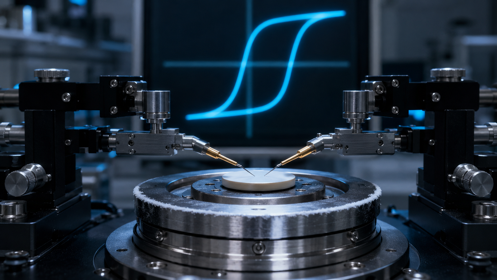
Drive a ferroelectric with a cyclic voltage and plot the polarization it develops against the applied field: the result is the hysteresis loop, and its anatomy is the vocabulary of the field. The saturation polarization Ps is the plateau where all domains have aligned; the remanent polarization Pr is what survives when the field returns to zero — the memory; the coercive field Ec is the reverse field needed to drag the net polarization back through zero — the cost of rewriting that memory. The classic circuit for recording it, published by Sawyer and Tower in 1930 for Rochelle salt, is elegance itself: the sample in series with a large known capacitor, so the big capacitor accumulates the sample’s switched charge and its small voltage reads out the polarization directly on an oscilloscope5. Modern ferroelectric testers refine the readout — virtual-ground charge integration, compensation, pulse sequences — but the object measured is the same: charge moved versus field applied.
Two disciplines make a loop quantitative. First, geometry: polarization is charge per electrode area, and field is voltage per thickness, so the electrode area and sample thickness enter every axis — measure them, and use electrodes with defined, complete coverage. Second, the drive itself is part of the result: loop shape depends on the field amplitude (an undersaturated “minor loop” reports smaller Pr and Ec than the material owns) and on frequency, because domain switching takes time. A reported loop therefore travels with its amplitude, frequency, waveform, temperature and electrode geometry — or it is decoration.
3. Bananas: Recognizing Fake Loops
Here is the trap that gives this field its cautionary classic. A lossy, leaky dielectric — with no ferroelectricity whatsoever — produces a fat, open, loop-shaped figure on the same axes, because leakage current integrated over a cycle masquerades as switched polarization. The point was made unforgettable by Scott’s “Ferroelectrics go bananas,” which noted that published “hysteresis loops” of this kind could be reproduced by materials as unferroelectric as a banana skin — lossy ionic conduction draws handsome cigar-shaped loops with no switchable polarization behind them6.
The forgeries have tells. A true ferroelectric loop shows concave saturation: beyond switching, polarization flattens toward Ps and the loop closes into slim tips. A leakage “banana” stays convex — rounded, cigar-like, fattening with drive amplitude and opening wider as frequency drops (more time per cycle for leakage charge to accumulate). The diagnostic toolkit follows from the physics: vary the frequency and watch whether the apparent Pr collapses; vary the amplitude and check whether the loop saturates or just inflates; and use switching-versus-non-switching pulse sequences — the PUND family — whose logic is to subtract the response of a pre-poled state (no switching, only leakage and linear dielectric response) from the response of a reversed state (switching plus everything else), leaving the genuinely switched charge67. A loop that shows credible saturation, appropriate frequency dependence and a consistent switching-minus-non-switching response provides strong evidence of switchable polarization; for difficult materials, combine these with switching-current peaks, retention, dielectric, pyroelectric or structural evidence as appropriate.
4. Piezoelectric Coefficients: What d33 Actually Means
The piezoelectric coefficients are the exchange rates between the electrical and mechanical worlds. The direct effect is charge per force: d33, the headline number, is the charge density generated along the poling axis per unit stress applied along that same axis, in pC/N. The converse effect is strain per field — and in linear piezoelectric constitutive theory, the direct and converse effects are described by the same tensor coefficient under matched definitions and boundary conditions. Practical measurements need not agree exactly: a Berlincourt-style quasi-static press, an interferometric displacement readout and a resonance method can differ because drive amplitude, frequency, clamping, preload, domain-wall contributions, field bias and calibration differ among them. The subscripts carry the geometry: d31 couples a field along the poling axis to strain perpendicular to it, the mode that bends bimorph actuators; shear coefficients get their own indices. Sign conventions, clamping conditions and frequency all matter, and the standard references catalogue how coefficients defined at constant stress versus constant strain differ1.
Two practical notes travel with any coefficient. First, in ferroelectric ceramics the measured d33 is not a fixed crystal constant: domain walls contribute an extrinsic share that depends on drive amplitude, bias, frequency, aging and — centrally for this article — temperature1. Second, piezoelectricity is not confined to ceramics: Kawai’s 1969 discovery of strong piezoelectricity in poled poly(vinylidene fluoride) opened the polymer branch8 — flexible, low-temperature materials whose modest coefficients and low Curie-region temperatures make temperature control not a luxury but the experiment itself.
The measurement family at a glance:
| Method | Measures | Extra hardware beyond the stage | Main caution |
|---|---|---|---|
| P–E loop | Polarization vs field | Ferroelectric tester | Leakage can mimic switching |
| PUND pulses | Switched vs non-switched charge | Pulse-capable tester | Timing; incomplete switching |
| Leakage I–V | Conduction current | Source–measure unit | Strongly temperature-dependent |
| Dielectric vs T | Permittivity and loss | LCR meter | Frequency dependence |
| Direct d33 | Charge per force | Controlled force + charge chain | Preload and frequency |
| Converse d33 | Strain per field | Displacement/strain sensor | Clamping; field uniformity |
5. Temperature, the Curie Point and Thermal Depolarization
Temperature is not a nuisance variable in ferroelectric testing; it is the second axis of the phase diagram. On warming toward the Curie temperature TC, the spontaneous polarization shrinks, the permittivity climbs toward a sharp peak, the coercive field softens, and at TC the polar phase surrenders to the nonpolar parent — the loop collapses into the slim, lossy curve of an ordinary dielectric. Above TC, the permittivity falls off with the Curie–Weiss behaviour that is the textbook signature of a vanished ferroelectric phase; barium titanate’s cascade of transitions on cooling — cubic to tetragonal to orthorhombic to rhombohedral, each with its own polar axis — is the canonical map of how much structure a “simple” ferroelectric can hide across a modest temperature range3.
For the working device community the operational quantity is thermal depolarization: a poled ceramic loses its aligned domain texture — and with it its piezoelectric coefficients — well before TC is formally reached, as thermal agitation lets domains relax toward disorder. The practical temperature limit for a poled element is material- and application-specific: it follows from the measured depolarization temperature Td (a distinct, lower landmark than TC), from d33 and polarization retention, from long-term aging under bias and stress, and from the manufacturer’s rated operating temperature — there is no universal fraction of TC that defines safe continuous use41. And it is exactly the kind of quantity a variable-temperature stage lets you replace with data: measure d33 or Pr after successive anneals at rising temperatures, and the material reports its own retreat schedule. The reverse direction matters too: poling is routinely performed warm, where the coercive field is soft, then locked in by cooling under field — a protocol that is impossible to do reproducibly without the ±0.1 °C class of stage control this article assumes.
6. Interactive: The P–E Loop Lab
The simulator below stages Sections 2, 3 and 5 in one canvas. It draws the polarization–field response of an illustrative ferroelectric as you vary two things: the sample temperature, from room temperature up through the model’s Curie point, and the leakage level, from insulating to lossy. The read-outs report the apparent remanent polarization and coercive field of whatever figure is on screen — and a schematic curvature-based shape check that warns when the figure looks leakage-convex rather than saturating — a teaching aid, not a complete ferroelectricity test.
Three lessons are built in. Warm the model toward its Curie point and watch Pr and Ec shrink together until the loop closes — the honest death of ferroelectric order. Raise the leakage on a cold sample and watch a fat convex banana inflate around the true loop — the apparent Pr climbs while the material’s actual memory has not changed at all, which is the entire Scott lesson in one slider. And the “Above TC + leaky” preset shows the most dangerous case: no ferroelectricity left whatsoever, yet the screen still shows a closed, loop-shaped figure. The model is schematic — a smooth switching function with temperature-scaled parameters and an ohmic leakage term — and its shape check inspects curvature at the field extremes, exactly the concave-versus-convex tell of Section 3.
7. The Error Budget: Where Ferroelectric Numbers Go Wrong
Leakage first, always. It is not merely a nuisance current; integrated over a cycle it adds directly to the apparent polarization, growing with measurement time and temperature — and leakage itself rises steeply on heating, so the banana risk is worst exactly where the Curie-point physics is most interesting6. Frequency variation and pulse subtraction belong in every warm campaign. Geometry second: P and E both carry the electrode area and thickness; fringing at small electrodes and incomplete coverage bias both axes. Then the drive: under-saturated minor loops understate Pr and Ec; excessive fields walk into breakdown — and dielectric strength falls with temperature, so the safe window narrows on heating. Self-heating closes the loop on itself: a lossy sample driven hard dissipates in exactly the volume being measured, shifting its true temperature above the stage reading — the small-sample trap in its dielectric costume9. And the temperature axis carries the usual terms — calibration against the practical scale, sample–stage offset, lag during ramps10 — with a ferroelectric-specific sting: near TC the properties change so steeply that a one-degree offset can move the measured transition and the peak permittivity visibly. Low-level measurement discipline — guarding, settling, averaging — is assumed throughout11.
8. A Testing Protocol: From Contact to Reported Loop
1. Verify the contacts and electrodes. Electrode area and coverage measured; contact I–V checked at both temperature extremes — the ferroelectric signal rides on the same contact physics as any transport measurement12.
2. Establish the leakage baseline. DC leakage versus field and temperature before any loop is trusted; it defines your banana risk.
3. Find saturation honestly. Loops at increasing amplitude until Pr and Ec stop growing; report the amplitude with the numbers.
4. Interrogate the frequency axis. Loops at two or three frequencies; a Pr that collapses at higher frequency was mostly leakage.
5. Confirm with pulse subtraction. A switching-minus-non-switching sequence isolates the truly switched charge7.
6. Then add temperature. Step-and-hold points per the companion methodology; at each setpoint, the full loop discipline; report Pr(T), Ec(T) and the criterion used for TC (loop closure, permittivity peak, or depolarization onset — they need not coincide) with amplitude, frequency, geometry and heating/cooling direction attached13.
9. Hardware Notes: Running This on a Stage
The experiments in this article assume stable, positionable electrical contact on a temperature-controlled platform: the InSitu Pro™ AECH600S / AECH400SV electrical stage supplies four movable probe holders with BNC feedthroughs and ±0.1 °C stability across −190 °C to 600 °C (air) or −190 °C to 400 °C (vacuum) — a range that covers the transition and depolarization regions of many common BaTiO₃- and PZT-based compositions and the operating and depolarization ranges of many polymer piezoelectric materials, with the usual caveat that stage stability is not sample accuracy. The division of labour deserves stating plainly: the stage provides the temperature environment and the electrical contacts for variable-temperature P–E, leakage and dielectric work when integrated with a compatible ferroelectric tester; direct d33 testing additionally requires a controlled force-and-charge measurement system, converse d33 a calibrated displacement or strain readout, and high-voltage poling its own safety and insulation design — none of which the temperature stage alone provides. Tester integration and high-voltage limits are configuration-specific and worth a quotation conversation; the OEM line explicitly supports ferroelectric-tester coupling on the electrical family. For the broader family and configuration matching, see the electrical stage line or the stage selector.
- Electrical Heating & Cooling Stage (AECH600S / AECH400SV) — the temperature environment and electrical contacts for variable-temperature P–E, leakage and dielectric work; ferroelectric-tester and d33-system integration by configuration.
- Variable-temperature electrical probe stages: the overview — contact physics, probe hardware and the measurement pitfalls this article builds on.
- Measuring R(T) in-situ — the leakage-resistance side of the same samples: fitting methodology and error budgets.
- All InSitu Pro™ electrical stages — the complete line, or use the interactive stage selector.
10. FAQ: Ferroelectric & Piezoelectric Testing
11. Keep Exploring the InSitu Pro™ Knowledge Hub
This article extends the electrical cluster of the InSitu Pro™ knowledge hub into functional materials. To keep going:
- In-situ heating, cooling & electrical stages: a theory guide — the pillar article on how temperature-controlled stages work.
- In-situ electrical probe stages — hardware, contacts and pitfalls for the whole electrical family.
- Resistance vs temperature: measuring R(T) in-situ — the fitting-methodology companion, including the leakage-resistance physics this article leans on.
- Four-probe & Hall measurements at variable temperature — geometries, field reversal and carrier extraction on the same platforms.
- How to choose an in-situ heating & cooling stage — the five-step selection guide.
References
This article discusses ferroelectric and piezoelectric measurement methodology in general terms. Loop parameters, coefficients, Curie temperatures, depolarization behaviour and the diagnostic criteria for distinguishing genuine switching from leakage artifacts are idealized and material-, geometry-, electrode-, drive- and instrument-dependent; real behaviour should be validated against the published literature, applicable standards, your own calibrations and the manufacturer’s datasheets before quantitative use. High-voltage ferroelectric testing carries electrical-safety obligations that are the operator’s responsibility. The interactive simulator is a schematic teaching tool — its loops are generated from a stated illustrative model, not from measured data — and is not a substitute for real ferroelectric characterization. Ferroelectric-tester integration on heating-and-cooling stages is configuration-specific; contact ACS Material to discuss options for your application.