
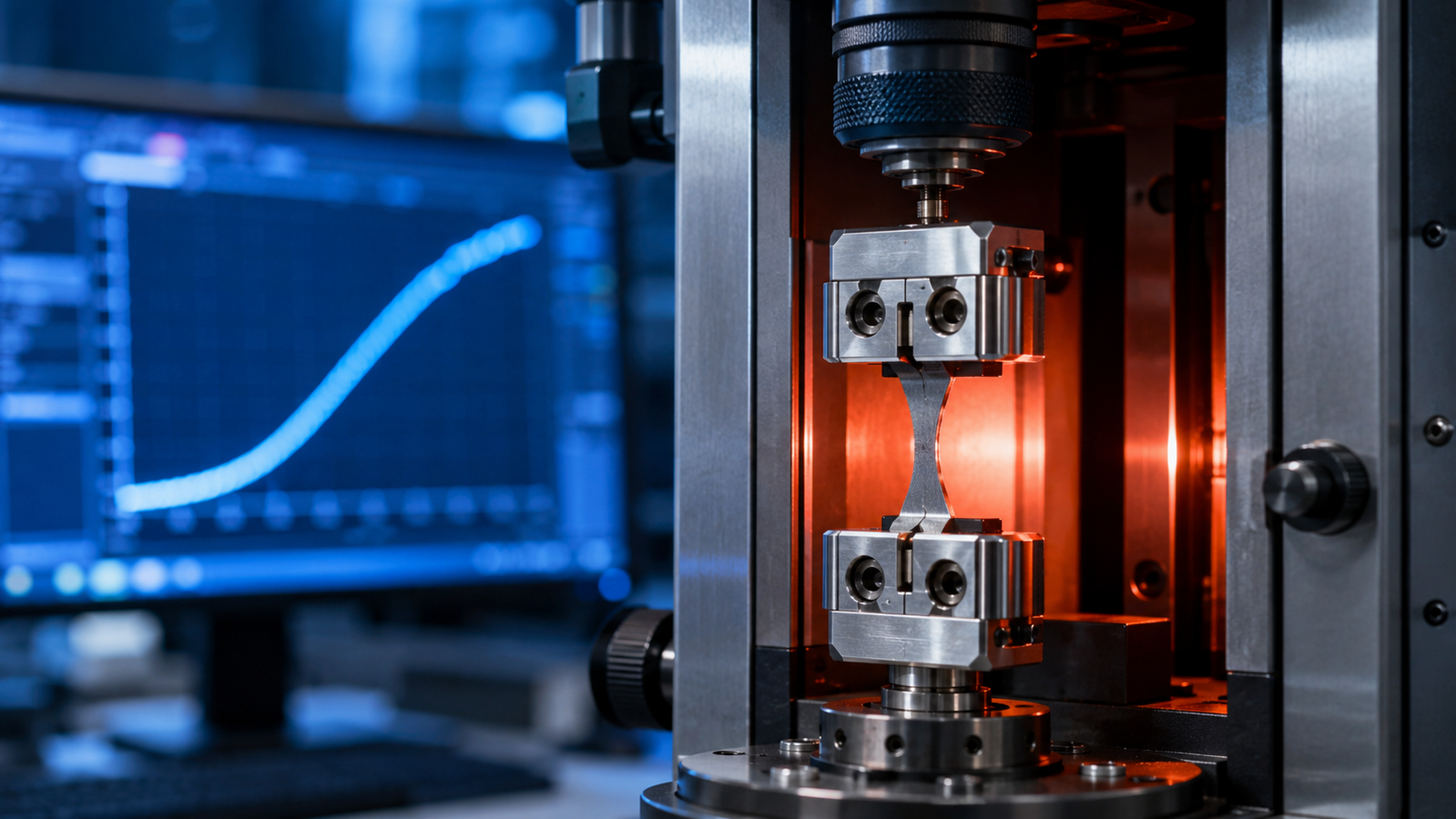
A stress–strain curve measured at room temperature describes a material that may never exist in service. Engines run hot, spacecraft run cold, and between those extremes elastic moduli soften, yield strengths retreat, ductility migrates, and whole deformation mechanisms switch on and off. In-situ tensile testing at variable temperature closes that gap twice over: it measures the mechanical response at the temperature that matters, and — because the frame sits under a microscope, a Raman objective or an X-ray beam — it lets you watch the microstructure earn every point on the curve. This article covers the anatomy of the curve, what temperature does to each of its landmarks, how strain is honestly measured when everything is expanding, and how to budget the errors. It is the first mechanical-testing chapter of the InSitu Pro™ knowledge hub, and it leans on the stage theory guide for everything thermal.
1. Why Pull In-Situ: Curve Plus Cause
A full-size universal testing machine delivers the curve; an in-situ stage delivers the curve and the reason for it. Mounted under an optical microscope, the stage shows slip bands forming, cracks nucleating at inclusions, and necks localizing in real time; under a Raman objective, stress maps onto peak shifts; in an X-ray beam, lattice strain and phase changes report from inside the bulk while the load cell reports from outside — the same correlative logic the hub’s in-situ XRD guide develops for structure and the SEM heating-stage guide develops for electron imaging. The second argument is scale: compact frames test the small specimens that modern materials actually come as — films, foils, fibers, additively built coupons, micro-machined dogbones — where a floor-standing frame is the wrong tool entirely; miniaturised-specimen testing now has its own specification in the same standards series1. The third is this article’s title: the temperature axis, because the mechanical properties being measured are themselves functions of temperature, often steep ones.
2. Anatomy of the Stress–Strain Curve
The engineering curve plots force over original cross-section (stress) against elongation over original gauge length (strain), and its landmarks carry the design handbook. The initial straight climb is elastic: its slope is Young’s modulus E, the stiffness, fully recoverable. Departure from the line marks yielding — reported as an offset yield strength (conventionally at 0.2% plastic strain) or, in materials with pronounced yield-point behaviour like mild steel, as upper and lower yield points with Lüders-band propagation between them, the phenomenon whose grain-size systematics Hall dissected in the 1951 papers that seeded the Hall–Petch relation2. Beyond yield, work hardening raises the flow stress as dislocations multiply and tangle; the peak of the engineering curve is the ultimate tensile strength (UTS) — and for a conventional ductile material under uniform quasi-static tension it commonly coincides with the onset of diffuse necking, though brittle fracture, damage or unstable localization can intervene earlier. Past the peak, deformation localizes and the engineering curve falls; in the conventional ductile picture the true stress in the neck continues to rise, though evaluating it there depends on local-area measurement and the damage state. Fracture ends the story. Uniform elongation (to the UTS) and total elongation (to fracture) are the two ductility numbers, and they answer different design questions. One bookkeeping habit prevents a family of mistakes: engineering stress and strain use original dimensions, true stress and strain use instantaneous ones, and the conversion matters exactly where curves get interesting — large strains and necks. Specimen geometry and procedure for all of this are standardized — by the ASTM E8/E8M family and by ISO 6892-1 for room-temperature metallic testing3 — and small-stage work follows the same logic at reduced scale.
3. What Temperature Rewrites: Every Landmark Moves
Temperature does not shift the curve; it rewrites it landmark by landmark. Stiffness: elastic moduli soften on heating — gently and quasi-linearly for most metals over hundreds of degrees — as the lattice’s restoring forces relax. Strength: yield and flow stress fall faster than stiffness, because plasticity in most metals is thermally activated — dislocations use thermal energy to defeat obstacles, so the stress required drops as temperature rises and climbs as it falls; the same physics makes flow stress rate-sensitive, and the coupled temperature–rate description is the business of thermal-activation constitutive frameworks such as the mechanical-threshold-stress model4. Ductility and mode: many ferritic steels and some other body-centered-cubic metals exhibit a pronounced ductile-to-brittle transition below a temperature range (the DBTT, named descriptively here) that depends on composition, microstructure, grain size, notch severity, strain rate and environment — turning a tough steel glassy in the cold, and making one of the sharpest arguments for testing cold rather than extrapolating. Mechanism handoffs: at sufficiently high homologous temperature — often around 0.4–0.5 Tm for many metals, depending on alloy, stress and timescale — creep and grain-boundary processes join the party and time enters the constitutive picture; polymers stage their own drama around the glass transition, softening by orders of magnitude across a few tens of degrees; shape-memory alloys reorganize their entire curve around martensitic transformation temperatures, trading plasticity for superelastic plateaus (described here descriptively). Even the “zero” moves: thermal expansion strains the specimen before any load is applied — and not always in the intuitive direction, as negative-thermal-expansion materials like ZrW₂O₈ contract on heating5 — so thermal and mechanical strain must be separated by protocol, not assumption. Low-temperature testing practice, from grip materials to instrumentation behaviour in the cold, is its own craft with its own standard references6.
4. Interactive: The Stress–Strain Lab
The simulator below draws the full engineering stress–strain curve of an illustrative metal as you move one slider: temperature, from deep cryogenic to red heat. A reference curve at room temperature stays on screen for comparison, and the read-outs report the four landmarks — modulus, 0.2% yield strength, UTS and uniform elongation — live as the material softens or stiffens under your finger.
Watch three things. Cold, the curve climbs: yield strength rises steeply (thermal activation withdrawn) while stiffness rises only slightly — the elastic slope and the yield plateau separate visibly. Hot, everything sags, but not in proportion: strength collapses faster than stiffness, and the hardening beyond yield flattens. And the model is honest about its edges: it is a smooth elastic–Hollomon-hardening construction with temperature-scaled parameters, truncated at a necking criterion — it contains no brittle fracture, no Lüders plateau, no creep and no transformation plasticity, which is precisely why the note under it says so. Real alloys add all four; the simulator teaches the baseline they add them to. One boundary matters commercially as well as scientifically: the simulator is a family-level teaching model extending to 500 °C — temperatures above 200 °C do not represent the AFCH500-200’s operating range, whose catalogued span is −190 °C to 200 °C; the high-temperature end of the family belongs to the 5000 N vacuum and SEM stages noted in the hardware section.
5. DIC vs Extensometer: Measuring Strain Honestly at Temperature
Force is the easy half — a calibrated load cell reads it. Strain is where variable-temperature testing earns its method section. Crosshead displacement, the tempting default, measures the whole mechanical chain: specimen, grips, frame compliance and every thermally expanding component between the motor and the gauge section — usable for comparative curves, misleading for moduli. Contact extensometers read the gauge section directly but must themselves survive and stay calibrated at temperature. The modern workhorse for in-situ stages is optical: digital image correlation tracks a speckle pattern on the specimen surface through the viewing window and returns full-field displacement and strain maps, with the two-dimensional formulation reviewed comprehensively by Pan and colleagues7. DIC’s full-field nature is not a luxury here — it is what lets you see strain localize into a neck or a Lüders front instead of averaging it away. Temperature adds DIC-specific homework: heat haze bends light above hot samples, speckle paints must survive the excursion, and radiant glow at high temperature demands filtering — solvable, and solved routinely, but only by protocols that name them. And whichever sensor is chosen, the thermal-strain bookkeeping of Section 3 applies: hold load near zero through a temperature change and let the measured strain report expansion — noting that this approximates free thermal strain only if grips, friction and the control loop let the gauge section expand with negligible constraint — and separate that record from the mechanical loading that follows.
The strain-measurement family at a glance:
| Method | Strength | Main error sources | Best use |
|---|---|---|---|
| Crosshead displacement | Simple, always available | Frame/grip compliance; thermal expansion of the chain | Comparative curve shapes |
| Clip-on extensometer | Direct gauge-section reading | Temperature rating; contact effects | Routine quantitative E and elongation |
| Digital image correlation | Full-field maps; sees localization | Speckle survival; heat haze; radiant glow | In-situ imaging; necking and Lüders fronts |
| Diffraction strain | Lattice strain from inside the bulk | Not the macroscopic total strain | XRD / synchrotron correlative work |
6. Thermal Strain, Machine Compliance and Measurement Error
The force axis: load-cell calibration and its temperature sensitivity; grip slippage, which forges fake strain and softens apparent moduli; misalignment, which bends what should be pulled and scatters brittle-material strengths. The strain axis: the compliance and expansion chain if displacement is used; extensometer calibration at temperature; DIC’s image-quality terms — speckle degradation, haze, glow7. The temperature axis: the specimen’s gauge section is what matters, not the enclosure air — gradients along a gripped specimen are the norm, not the exception, and the calibration chain runs back to the practical scale as everywhere else in this hub8. The definitional terms: original-versus-instantaneous dimensions, offset conventions for yield, and rate: flow stress depends on strain rate through the same thermal activation that makes it depend on temperature4, so rate is a reported condition, not a footnote. The formal evaluation of tensile-testing uncertainty has its own technical-report literature9. The blunt summary mirrors the electrical cluster’s: tensile uncertainty is usually systematic — compliance, gradients, slippage, definitions — and the systematics deserve the effort before the noise does.
7. A Testing Protocol: From Mounting to Reported Curve
1. Know the specimen. Gauge dimensions measured, not assumed; geometry per the relevant standard family — room-temperature procedure per ISO 6892-1 / ASTM E83, elevated-temperature per ISO 6892-210, low-temperature (down to −196 °C) per ISO 6892-311 — scaled honestly for the stage.
2. Align and grip deliberately. Verify with a low-load elastic cycle: hysteresis or offset flags slippage or misalignment before they cost a specimen.
3. Separate thermal from mechanical strain. Reach temperature at near-zero load; record the thermal-strain baseline; only then load.
4. Soak before pulling. Hold at setpoint until the gauge section — not the controller — is stable; small stages equilibrate fast, but “fast” is measured, not assumed.
5. Pull at a named rate. Constant crosshead or strain-rate control, stated with the curve; if rate sensitivity is the question, bracket it deliberately.
6. Report the conditions with the landmarks. E, yield (with offset convention), UTS, elongations — each with temperature, rate, strain-measurement method, specimen geometry and atmosphere. The reproducibility test is the usual one: a stranger with your raw force–displacement record and metadata reaches your numbers unaided.
8. Hardware Notes: Running This on a Stage
The platform this article is written around is the InSitu Pro™ AFCH500-200 desktop tensile stage: a compact heated-and-cooled tensile frame built to sit under observation optics, marrying the load frame to the same temperature-control discipline as the rest of the InSitu Pro™ family. Its catalogued specification is concrete: −190 °C to 200 °C at ±0.1 °C (liquid-nitrogen cooling + resistive heating), two tensile-force ranges of 20 N and 500 N each at 0.5% F.S. accuracy, 100 mm of displacement travel at 0.1–100 mm/min, interchangeable fixtures for tension, compression, shear and bending, an atmosphere chamber over a 35 × 12 mm silver stage, and a φ45 × 1 mm quartz window for the microscope — with sensor, fixture and any alternative-chamber configuration confirmed at quotation. For work the desktop model does not cover, the same family scales up: the AFH5000-1000V carries 5000 N (0.5% F.S., 20 mm travel) from room temperature to 1000 °C in a vacuum chamber, and the ASFH5000-1200 carries 5000 N (0.1% F.S., 10 mm travel) to 1200 °C built for SEM chambers — the high-temperature branch the simulator’s >200 °C region belongs to. The correlative pairings write themselves: optical microscopy for surface mechanisms, Raman for stress spectroscopy, XRD for lattice strain and phase evolution, SEM modules for electron-microscope integration. For matching a mechanical stage to the rest of an experiment, the stage selection guide walks the decision and the stage selector filters the family.
- Desktop Tensile Stage (AFCH500-200) — −190 to 200 °C, 20/500 N at 0.5% F.S., four mechanical modes: the compact frame this article’s protocols are written for.
- In-situ XRD: watching crystal structure evolve — the diffraction partner for lattice strain and stress-induced phase changes.
- In-situ SEM heating stages — electron-microscope integration for watching deformation mechanisms at magnification.
- How to choose an in-situ stage — the five-step selection guide, or go straight to the interactive stage selector.
9. FAQ: In-Situ Tensile Testing
10. Keep Exploring the InSitu Pro™ Knowledge Hub
This article opens the mechanical-testing wing of the InSitu Pro™ knowledge hub. To keep going:
- In-situ heating, cooling & electrical stages: a theory guide — the pillar article on temperature control, lag and stability that every stage in the family shares.
- In-situ XRD: watching crystal structure evolve — lattice strain, phase transitions and diffraction under stimulus.
- In-situ SEM heating stages — watching dynamics live in the electron microscope.
- Variable-temperature Raman spectroscopy — the vibrational partner: stress and temperature written into peak positions.
- How to choose an in-situ heating & cooling stage — the five-step selection guide with interactive simulators.
References
This article discusses variable-temperature tensile testing methodology in general terms. Curve landmarks, temperature dependences, transition behaviours and strain-measurement performance are idealized and depend on material, microstructure, specimen geometry, gripping, rate, atmosphere and instrumentation; real values must be established experimentally and validated against the relevant standards, the published literature, your own calibrations and the manufacturer’s datasheets before quantitative use. The interactive simulator is a schematic teaching tool — a stated illustrative constitutive construction, not measured data for any real alloy — and deliberately omits brittle fracture, yield-point phenomena, creep and transformation plasticity. Tensile-stage specifications — load capacity, temperature range, grips, clearances — are configuration-specific; contact ACS Material to discuss options for your application.