Every materials lab owns instruments that answer the question what is this sample like? — microscopes, spectrometers, diffractometers, probe stations. An in-situ stage upgrades the question to what is this sample doing? It is a compact, instrument-mounted environment that holds your sample at a chosen temperature — from deep cryogenic to furnace-hot — sometimes under a chosen atmosphere, sometimes with electrical contacts, while your existing instrument watches. This beginner’s guide is the front door to the InSitu Pro™ knowledge hub: what a stage actually is, the three stimuli it delivers, what happens inside the little chamber, and how to tell whether your experiment is one of the many that quietly need one.
1. Why “In Place” Matters
Most characterization is before-and-after: prepare a sample, treat it somewhere else, bring it back, measure what survived. The gap in the middle is where the science leaks out. Transient states relax, hot phases transform on cooling, surfaces react with air on the walk between furnace and microscope — and the measurement reports the survivor, not the process. The in-situ idea is old and simple: put the environment on the instrument so nothing has to survive a journey. It has a distinguished pedigree — X-ray diffraction of a battery electrode was recorded during electrochemical cycling as early as 19781 — and a spectacular modern showcase: environmental electron microscopy has watched catalyst nanoparticles oscillate between shapes in real time under reaction gas, dynamics that no before-and-after pair of images could ever have revealed2. The stage is how that philosophy arrives on an ordinary lab bench.
2. Three Core Controls: Temperature, Environment, and Applied Stimulus
Heat is the universal accelerator and transformer: melt, crystallize, anneal, oxidize, sinter, decompose — nearly every materials process has a temperature axis, and heating stages make it visible from just above ambient to furnace territory. Cold is the other half of the axis and often the more surprising one: phases freeze into observability, thermal noise quiets, and entire phenomena exist only below room temperature — the classic metal–insulator switch in vanadium dioxide flips near a comfortable 68 °C, but its low-temperature cousin phases and much of correlated-electron physics live far colder3. Even thermal expansion misbehaves informatively: some materials contract on heating, and only a variable-temperature measurement catches them doing it4. Electricity turns observation into interrogation: with contacts or probes inside the chamber, the stage measures resistance, ferroelectric response or device behaviour as a function of the temperature it controls — the combination the electrical wing of this hub is built on. Most stages deliver one or two of these controls; the family as a whole spans temperature, environment and applied stimulus — with atmosphere control and mechanical loading extending the same logic in the deeper chapters.
3. Anatomy of a Stage: What’s Inside the Little Box
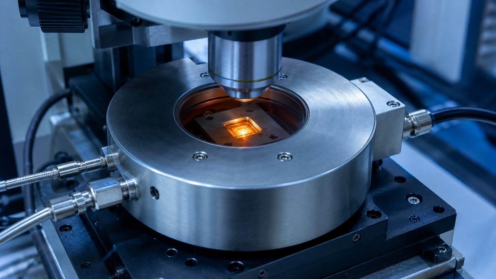
Strip any stage to its skeleton and up to five recurring elements remain. A temperature-controlled sample platform — typically a metal block heated electrically and cooled by liquid nitrogen or a thermoelectric element — that the sample sits on. A sensor and controller closing the loop, holding the platform to the setpoint within tight stability bands; every temperature claim ultimately traces to a calibration chain anchored in the international temperature scale5. Around it, a sample environment that, depending on the model, may be open, atmosphere-enclosed, vacuum-capable, or configured for a confirmed gas-flow arrangement — sealed or dry-purged where frost-controlled cryogenic work requires it. An optical or X-ray window where beam access is required — matched to the instrument: optically flat for microscopy, Raman-quiet for spectroscopy, X-ray-transparent for diffraction. And feedthroughs where needed — gas lines, electrical contacts, probe access. One honest caveat belongs in the beginner’s tour: the controller reports its sensor, and the sample can differ from it — through lag after setpoint changes, through gradients, and even through self-heating when the sample itself dissipates power6. The pillar article dissects that gap; the habit to form on day one is simply to respect it.
4. Interactive: The Setpoint Step & Follow Lab
The simulator below shows the stage’s core job in one control. Move the setpoint and watch two curves: the program the controller commands, and the sample temperature following it with a short lag — the fundamental physics every article in this hub builds on.
Two lessons hide in the simple picture. The sample always arrives a little after the program — so “measure at 300 °C” really means “wait until a validated sample-temperature reading or an established equilibration criterion says the specimen has settled”. And the faster the ramp, the larger the momentary gap between command and reality — the origin of the soak times, stability specs and ramp-rate trade-offs the rest of this hub treats in depth. The model is a schematic first-order step response with a teaching time constant — not a full programmed-ramp simulation, and not data for any real stage.
5. A Short History of Watching Materials Change
The idea of watching materials change is far older than the hardware that now makes it routine, and a short genealogy explains why the modern stage looks the way it does. The founding gesture of the field was made with X-rays: in 1978, diffraction patterns were recorded from a battery electrode while it charged and discharged, proving that structural chemistry could be read live from a working system rather than reconstructed from autopsies1. Four years later, a different revolution made the point at the atomic scale — the scanning tunneling microscope showed that surfaces could be imaged atom by atom, and its descendants quickly learned to do so while those surfaces were heated, cooled and reacted7. The lesson of both milestones was identical: the instrument does not have to wait for the process to finish.
Two further waves brought the philosophy to every bench. The materials boom of the 2000s — symbolized by the isolation of graphene and the two-dimensional materials program it launched — created an enormous population of samples whose properties are exquisitely temperature-dependent, and whose characterization therefore demands a temperature axis as a matter of course8. And environmental electron microscopy supplied the era’s defining images: catalyst nanoparticles filmed oscillating between shapes under reaction gas, dynamics that exist only while the environment does2. What was once a specialist’s trick at a national facility became a product category — the compact, instrument-mounted stage — and the barrier to entry fell from a beamline proposal to a purchase order. The rest of this hub is, in a sense, the user manual for that historical arrival.
6. Five Classic Experiments to Run in Week One
Abstractions convince slowly; experiments convince fast. Here are five classics, each runnable in a first week with a stage and an instrument you already own, and each a doorway into a chapter of this hub. One: melt and grow a polymer. Take a semicrystalline polymer film between crossed polarizers, melt it, and cool at a controlled rate — spherulites nucleate and grow before your eyes, and changing the cooling rate visibly changes the microstructure you make. It is the fastest possible demonstration that processing history is written in morphology. Two: watch steel change color. Heat a polished steel coupon in air and watch temper colors sweep across the surface as the oxide film thickens — interference turning film growth into a visible clock, and the gateway experiment to quantitative oxidation work.
Three: switch vanadium dioxide. A VO₂ film crossed slowly through ~68 °C snaps from insulator to metal within a degree or two — watch it optically or electrically, then map the hysteresis by cycling both directions; it is the canonical sharp transition and the perfect first test of your stage’s stability discipline3. Four: chase a polymorph. Heat a polymorphic pharmaceutical compound on the hot stage and catch the solid-state conversion — a needle-to-plate recrystallization, a melt-and-recrystallize sequence — the observation that founded an entire regulatory science of drug forms9. Five: measure your own device’s fever. Put a powered device on the stage and compare its behaviour against platform temperature with the power on and off — self-heating made visible, the everyday reality that thermal metrology of working electronics is built on10. Five afternoons; five chapters of this knowledge hub opened with your own hands.
7. Which Instruments It Serves
The stage is a chameleon: the same core mounts under very different eyes. Under an optical microscope it turns melting, crystallization and oxidation into movies. Under a Raman spectrometer it adds a temperature axis to every spectrum — with full-field optical strain techniques joining in where mechanics matter11. On an X-ray diffractometer it watches crystal structures evolve pattern by pattern. On a probe station it makes every electrical measurement a function of temperature. And in an electron microscope, purpose-built heating stages carry the same idea to the nanoscale. Each pairing has its own chapter in this hub — the window materials, the geometries, the error budgets — but the concept never changes: one controlled environment, many instruments.
8. What You Can Actually Watch
A sampler from across the hub, to make the abstraction concrete. Transformations: a polymer melting and recrystallizing into spherulites under crossed polarizers; a pharmaceutical switching polymorphs on a heating ramp. Reactions: a metal surface coloring as its oxide thickens in air; a catalyst working under reaction gas. Transitions: vanadium dioxide snapping from insulator to metal within a degree or two3; superconductivity appearing as resistance vanishes on cooling. Function: a ferroelectric’s hysteresis loop fattening and collapsing with temperature; a battery electrode’s lattice breathing with charge. None of these is a before-and-after pair — each is a process, and the stage is the ticket to watching it.
9. Reading a Stage Datasheet: A Beginner’s Decoder
Sooner or later the beginner meets a datasheet, and the numbers land better with a decoder ring. Temperature range is the headline, but read it as two numbers with separate price tags: the cold limit names the cooling technology (and its logistics), the hot limit names the construction class (and its window and atmosphere consequences) — the temperature-ranges guide in this hub maps both directions. Stability describes how tightly the controlled temperature stays within a band once settled — many precision optical and electrical stages specify values as tight as ±0.1 °C, while application-specific and ultra-high-temperature platforms publish different figures. Tight stability is a key contributor to resolving narrow thermal events, though it is distinct from display resolution, absolute accuracy, sample uniformity and overall measurement uncertainty; treat it as a scientific specification, not a luxury. Ramp rate is kinetic reach in both directions — the top speed for outrunning processes, and, just as valuably, the controlled crawl for crossing events slowly. Accuracy is a different animal from stability: stability says the temperature holds still, accuracy says the number is true, and the second rides on a calibration chain anchored in the international temperature scale5.
The remaining lines describe the meeting between stage and instrument. Window material and aperture decide what your probe sees and through how much glass — optical flatness for imaging, spectral quietness for Raman, X-ray transparency for diffraction; the dedicated windows chapter of this hub is the deep dive. Working distance and geometry decide whether your objectives physically fit. Atmosphere and vacuum options decide whether the chamber can be purged, sealed or pumped — the door to the oxidation, catalysis and frost-free-cryo work described elsewhere in this hub. And sample size and mounting decide the thermal contact everything above depends on. A beginner’s reading order: range first (does it reach my science?), stability second (does it resolve my events?), window and geometry third (does it fit my instrument?) — and let the selection guide arbitrate the ties.
10. Do You Need One? A Short Diagnostic
Ask three questions of your current workflow. Do you heat or cool samples somewhere else, then carry them to the instrument? Every carry is a relaxation window and an air exposure — a stage removes the journey. Do any of your plots have temperature on the x-axis? If you assemble them point-by-point from separate treatments, a stage turns days of that into one programmed run. Do you suspect the interesting state doesn’t survive to the measurement? Metastable phases, transient intermediates, working states — that suspicion is usually correct, and in-situ observation is the standard remedy. If any answer is yes, the next stop is the five-step selection guide or the interactive stage selector; the InSitu Pro™ family spans the optical, spectroscopy, diffraction, electrical and SEM configurations this hub’s chapters describe.
11. FAQ: In-Situ Stage Basics
12. Keep Exploring the InSitu Pro™ Knowledge Hub
This article is the front door of the InSitu Pro™ knowledge hub. To keep going:
- In-situ vs ex-situ characterization — the methodological case for watching it happen.
- In-situ heating, cooling & electrical stages: a theory guide — the pillar article on how temperature control really works.
- How to choose an in-situ heating & cooling stage — the five-step selection guide.
- Hot-stage microscopy — the optical chapter: melting, crystallization and more under the objective.
- In-situ XRD: watching crystal structure evolve — the diffraction chapter.
- All InSitu Pro™ stages — the complete family, or jump to the interactive stage selector.
References
This article introduces in-situ stages and their applications in general terms. Capabilities, temperature ranges, stability figures and compatibility are model- and configuration-specific; consult the applicable product datasheets and the published literature, and validate against your own instruments and calibrations before quantitative use. The interactive simulator is a schematic teaching tool built on a stated first-order lag model, not measured data for any real stage. Contact ACS Material to discuss configurations for your instrument and application.