
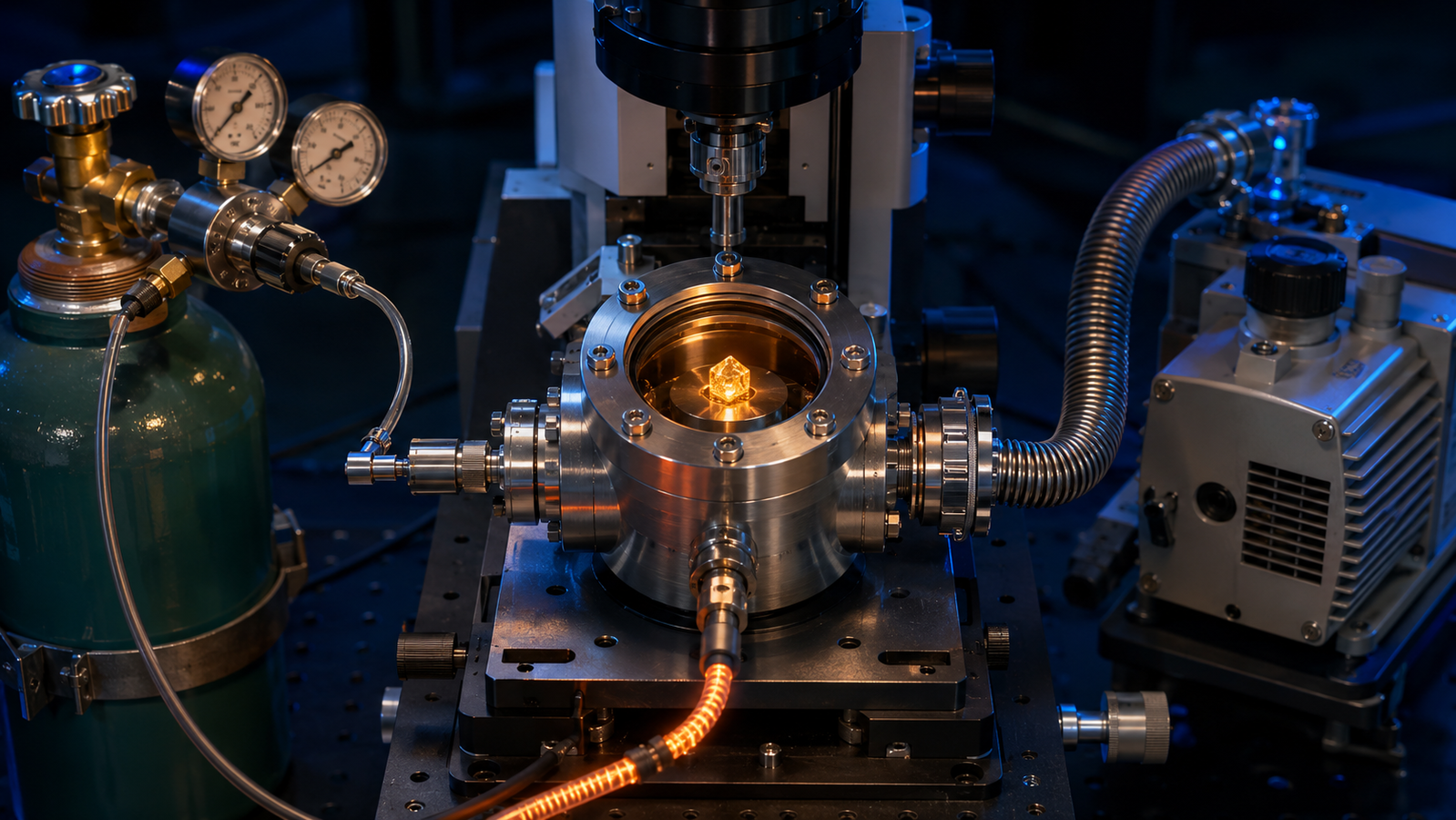
Room temperature, laboratory air, atmospheric pressure: the default environment of every instrument, and one that most of materials science does not actually live in. Batteries cycle warm, catalysts convert in reaction gas, alloys serve in the cold, coatings grow in vacuum, oxides form in air the moment you stop preventing it. Non-ambient characterization is the umbrella term for measuring outside the default — and it stands on three pillars that this article takes one at a time: temperature, the axis everything depends on; atmosphere, the silent reactant in every hot experiment; and vacuum, the environment of removal. Understand the three, and every specialized chapter in this hub becomes a variation on a theme.
1. Pillar I: Temperature — The Master Axis
Temperature is the non-ambient axis with no bystanders: many thermally activated rates accelerate with it, and temperature is a principal axis of many phase diagrams, every material eventually transforms along it. In characterization terms it is also the best-behaved axis — continuously tunable from cryogenic to furnace territory, precisely controllable, and traceable through a formal calibration chain to the international temperature scale, which is what allows two laboratories’ “300 °C” to mean the same thing1. The non-ambient diffraction tradition grew up around this axis first — heated and cooled sample chambers on diffractometers, with a methodological literature all their own2 — and this hub’s pillar article dissects its fine print: setpoint versus sample, lag, gradients, stability. For this overview, one sentence carries the essence: temperature is the axis you will always be using; the other two decide what happens while you do.
2. Pillar II: Atmosphere — The Silent Reactant
Heat a metal in laboratory air and you are not running one experiment but two: the thermal process you intended, and an oxidation reaction you didn’t order. Air is a reactant — at high temperature an aggressive one, growing oxide scales whose kinetics follow their own laws, from the parabolic thickening of protective scales to the logarithmic regimes of thin films3, a field mapped comprehensively by the high-temperature oxidation literature4 and, at the thin-film end, by the classic silicon oxidation framework5. Atmosphere control turns this from contamination into a dial with four settings. Inert (nitrogen, argon): suppress most oxidation and reaction pathways so the thermal process dominates — residual oxygen, moisture, outgassing and material-specific gas reactions remain part of the experiment. Oxidizing (air, oxygen): make the reaction the experiment — the deliberate business of in-situ oxidation studies6. Reducing or reactive (hydrogen mixtures, reaction feeds): drive chemistry the sample will meet in service, the doorway to catalysis work. Humidity-controlled: for hydrates, corrosion and everything water touches. For controlled-flow work, a compatible atmosphere or reaction cell commonly provides defined gas inlet and outlet paths; other non-ambient experiments use open stages, static-atmosphere chambers, sealed cells or vacuum configurations as the application demands — the science is choosing the setting deliberately.
3. Interactive: The Atmosphere Switch Lab
The simulator below makes Pillar II tactile. One sample, one temperature slider, one atmosphere toggle: watch the oxidation mass-gain curve grow parabolically in air, accelerate steeply with temperature, and collapse to near-nothing under inert purge — the same thermal history, two entirely different experiments.
Two build-in lessons. The temperature dependence is exponential — a modest temperature increase multiplies the parabolic rate constant, which is why “a bit hotter” can mean “visibly oxidized”. And the inert curve is suppressed, not zero: real purges carry residual oxygen, so demanding work speaks in purity grades and flow rates rather than absolutes. The model is a schematic parabolic law with an Arrhenius rate constant and teaching parameters — not data for any real metal.
4. The Science of Scale Growth
Because atmosphere’s chief business at temperature is scale growth, the serious reader deserves the theory one level deeper than “parabolic.” The canonical mechanism is diffusion control: once a continuous oxide film covers the metal, further growth requires ions or electrons to cross it, the film’s own thickness becomes the resistance, and the growth rate falls as the reciprocal of thickness — integrate that and the parabolic law Δm² ∝ t emerges. Wagner’s classical treatment put this on quantitative footing, tying the parabolic rate constant to the defect chemistry and ionic transport of the oxide itself — the reason different oxides protect so differently7. The framework explains the practical hierarchy every metallurgist knows: scales that grow slowly are scales that transport slowly, and alloying for oxidation resistance is largely the art of arranging for such a scale to form and stay adherent4.
The parabolic law is the middle of the story, not the whole of it. At the thin-film limit — the first nanometers, and low temperatures — electric fields set up across the nascent film drive ion transport and produce the logarithmic and inverse-logarithmic laws of the Cabrera–Mott regime3; the same conceptual territory, translated to semiconductor technology, yields the linear-parabolic framework that governed silicon oxidation for a generation5. And when scales crack, spall or form volatile species, protection collapses into linear or worse kinetics — breakaway oxidation, the failure mode high-temperature design guards against. For the in-situ observer the taxonomy is a field guide: the shape of your live mass-gain or color-front curve is a mechanistic clue — strongest when combined with phase, morphology, oxygen-partial-pressure dependence, activation energy and independent thickness or mass-gain checks — and watching the kinetics change regime — logarithmic to parabolic, parabolic to breakaway — is precisely the kind of event that endpoint measurements interpolate past6.
5. Pillar III: Vacuum — The Environment of Removal
Vacuum is atmosphere control taken toward its logical end: reduce total pressure and the partial pressures of reactive species until residual gases, outgassing, leaks and sample-generated vapour are what remain of the atmosphere. Three motives recur. Protection at temperature — with reactive partial pressures driven far down, many samples can be taken hot with scaling strongly suppressed (residual O₂/H₂O, outgassing and contamination still set the floor); vacuum and inert-purge chambers are the standard armor of high-temperature diffraction8. Instrument necessity — electron microscopes and many spectroscopies simply require vacuum for their beams to travel, making it the entry fee rather than a choice, with its own physics of beam–sample interaction to respect9. Process realism — thin-film growth, outgassing and space-environment studies are vacuum processes, and characterizing them means joining them there; laboratory in-situ instruments increasingly build the pumping in10. The costs are candid: vacuum strongly suppresses gas convection as pressure falls (changing every thermal calculation), encourages evaporation of volatile components, and adds windows, seals and pumps to the error budget. Some purpose-built multi-environment cells combine the three axes for programs that need them in one holder11.
6. Vacuum Processes as Experiments
Vacuum entered this article as protection and as an instrument’s entry fee; its third identity is the most interesting: vacuum as the process environment itself, with characterization joining the process where it lives. Many functional thin films are deposited under vacuum or controlled low-pressure environments — sputtered, evaporated and plasma-deposited films for optics, electronics and wear protection — and the properties of those films are set by what happens at the growing surface under process pressure and flux; the optical-coatings tradition documents in detail how deposition environment writes itself into film density, stress and index12. Characterizing such materials at ambient afterwards answers “what was made”; characterizing them in vacuum, at process-like temperature, moves the question usefully closer to “what is being made.”
The same logic runs in reverse for material removal: plasma etching — up to its atomically precise modern limit of atomic layer etching — is likewise a vacuum-chamber craft whose mechanisms are studied under the pressures and chemistries where they operate13. For the stage user the practical translations are concrete. Outgassing studies — what a polymer, adhesive or composite releases on heating in vacuum — are native vacuum experiments with direct consequences for space hardware and semiconductor tooling. Sublimation and evaporation, suppressed at atmospheric pressure, become active mass-loss channels the moment the pressure drops, which is both a hazard to plan for and a phenomenon to study. And the thermal bookkeeping changes wholesale: with gas convection strongly suppressed, the radiative and conductive terms carry everything, which is why a vacuum-capable stage’s calibration is verified in vacuo rather than inherited from gas — the cross-axis discipline this article’s error-budget section formalizes.
7. Combining the Axes
Real experiments live at coordinates, not on axes. Sintering studies run hot + inert to watch densification without oxidation. Oxidation kinetics run hot + controlled oxygen to make the reaction quantitative. Catalysis runs hot + reactive flow, ideally with products analyzed downstream — the operando coordinate. Cryogenic work runs cold + dry purge, because the atmosphere problem inverts below the dew point: the enemy is no longer oxidation but frost. Battery cells run warm-to-cold + sealed, their own electrolyte as the atmosphere. The craft of non-ambient design is naming your coordinate before choosing hardware — which is exactly the ordering the selection guide in this hub enforces.
8. Instrument by Instrument: The Pillars in Practice
The three pillars land differently on each instrument, and a quick tour grounds the abstractions. Optical microscopy is the most forgiving host: windows are often accommodated readily, but atmosphere, gas-flow, sealing and vacuum capability depend on the stage architecture and must be verified by model and configuration; the oxidation and hot-stage chapters of this hub live here. Raman spectroscopy inherits the optical geometry but adds spectral demands: the window must be quiet where your peaks live, and laser heating joins the error budget — atmosphere control matters doubly because a purge that prevents oxidation also protects against laser-accelerated reactions at the illuminated spot. X-ray diffraction is the historical home of the full triad: non-ambient chambers spanning furnace heat, controlled gas and vacuum were built for diffractometers early and refined into a documented methodology2, with the high-temperature end — reactive samples in inert or vacuum environments — a specialty of its own8.
Electron microscopy inverts the logic: vacuum is not an option but the native condition, atmosphere becomes the engineering achievement (differential pumping and windowed cells admitting gas at the sample), and beam–sample interaction joins temperature in the error budget as a first-class term9. Electrical probing, finally, adds feedthroughs to whichever environment it inhabits — contacts that must survive the temperature, resist the atmosphere, and not become thermal short-circuits into the sample. The practical use of this tour is triage: your instrument determines which pillars are cheap, which are engineered, and which are the experiment’s real constraint — knowledge worth having before the selection guide asks you to name your coordinates.
9. The Hardware Landscape
The InSitu Pro™ family maps onto the three pillars directly. Temperature is the family’s spine — heating, cooling and combined stages across the range the temperature-ranges guide describes. Atmosphere capability varies by model — open, atmosphere-enclosed and confirmed gas-flow configurations across optical, spectroscopic and diffraction stages — the configurations behind this hub’s oxidation and catalysis chapters. Vacuum capability appears both as vacuum-tight stage options and in the electron-microscope stages that live in vacuum by profession. Which combination your experiment needs is a coordinates question — the five-step selection guide walks it, the interactive stage selector shortcuts it, and atmosphere/vacuum options are confirmed per model at quotation.
10. The Cross-Axis Error Budget
Each pillar adds terms; the combinations multiply them. Temperature: the sensor–sample gap in all its forms — lag, gradient, calibration — anchored by traceability1. Atmosphere: residual reactive gas in “inert” purges; flow-induced temperature disturbance; window transmission changing as deposits form. Vacuum: the suppression of gas convection rewriting thermal contact (a sample that read true in gas can run hot in vacuum); evaporation and redeposition; pressure gauges with their own calibration chains. Cross terms: gas composition altering heat transfer and hence the effective calibration; frost as the cold-side atmosphere failure; beam effects amplified when convective cooling is absent9. The universal remedy repeats across this hub: verify at the sample, in the actual environment, not at the controller in the assumed one.
11. FAQ: Non-Ambient Basics
12. Keep Exploring the InSitu Pro™ Knowledge Hub
This article is the environmental map of the InSitu Pro™ knowledge hub. To keep going:
- In-situ heating, cooling & electrical stages: a theory guide — Pillar I in depth.
- In-situ oxidation studies by optical microscopy — Pillar II turned into the experiment.
- Catalysis in-situ: reactions under gas & heat — the reactive-atmosphere frontier.
- In-situ SEM heating stages — where vacuum is the native environment.
- In-situ XRD: watching crystal structure evolve — non-ambient diffraction in practice.
- How to choose an in-situ stage — from coordinates to hardware.
References
This article discusses non-ambient characterization in general terms. Oxidation kinetics, purge residuals, vacuum effects and calibration transfer are material-, hardware- and configuration-specific; validate against the published literature, applicable datasheets and your own measurements before quantitative use. The interactive simulator is a schematic teaching tool built on a stated parabolic-Arrhenius model, not data for any real material. Atmosphere and vacuum options vary by stage model; contact ACS Material to discuss configurations for your application.